Philharmonic BMR Bookshelf Speaker Review

Saturday, Jul 18, 2020

YouTube Video Review version:

Intro

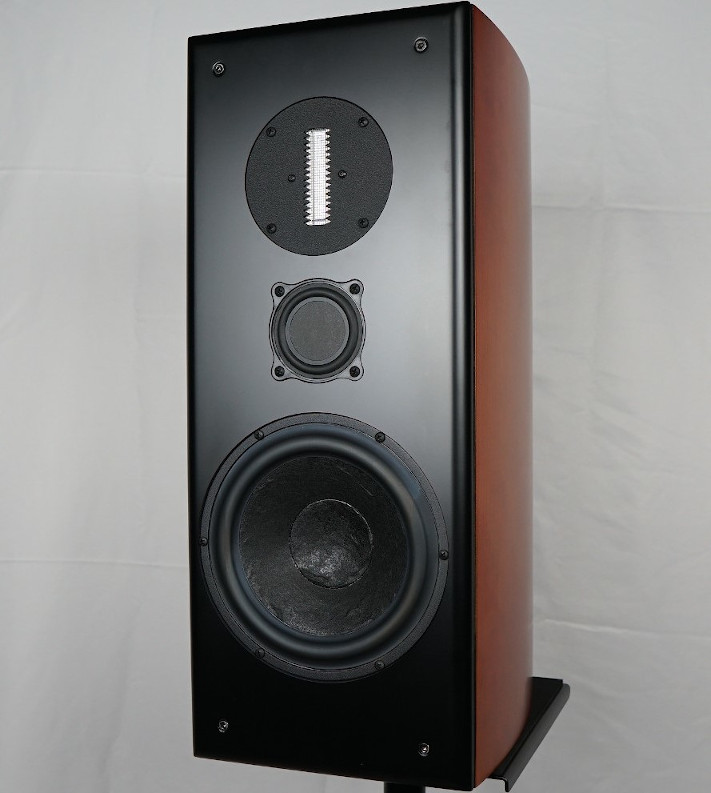
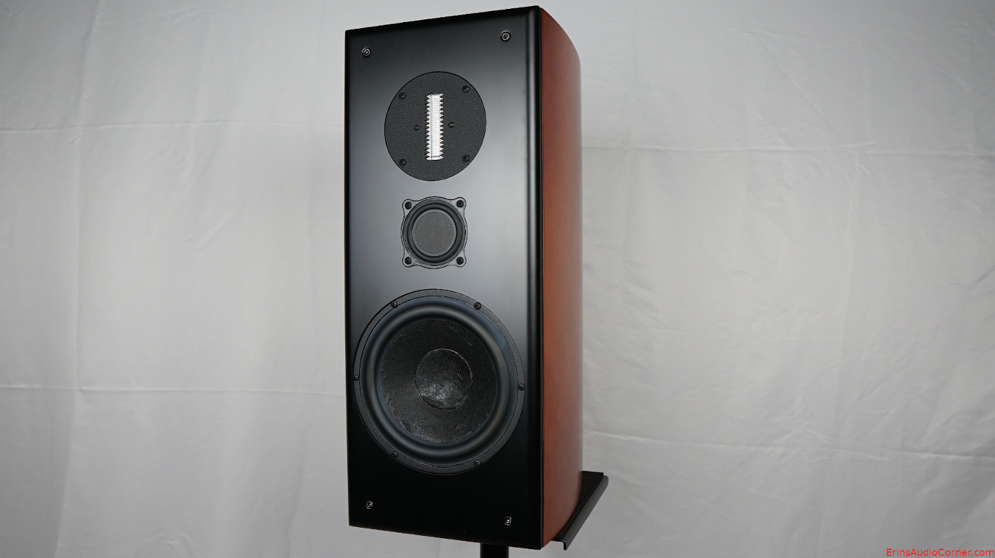
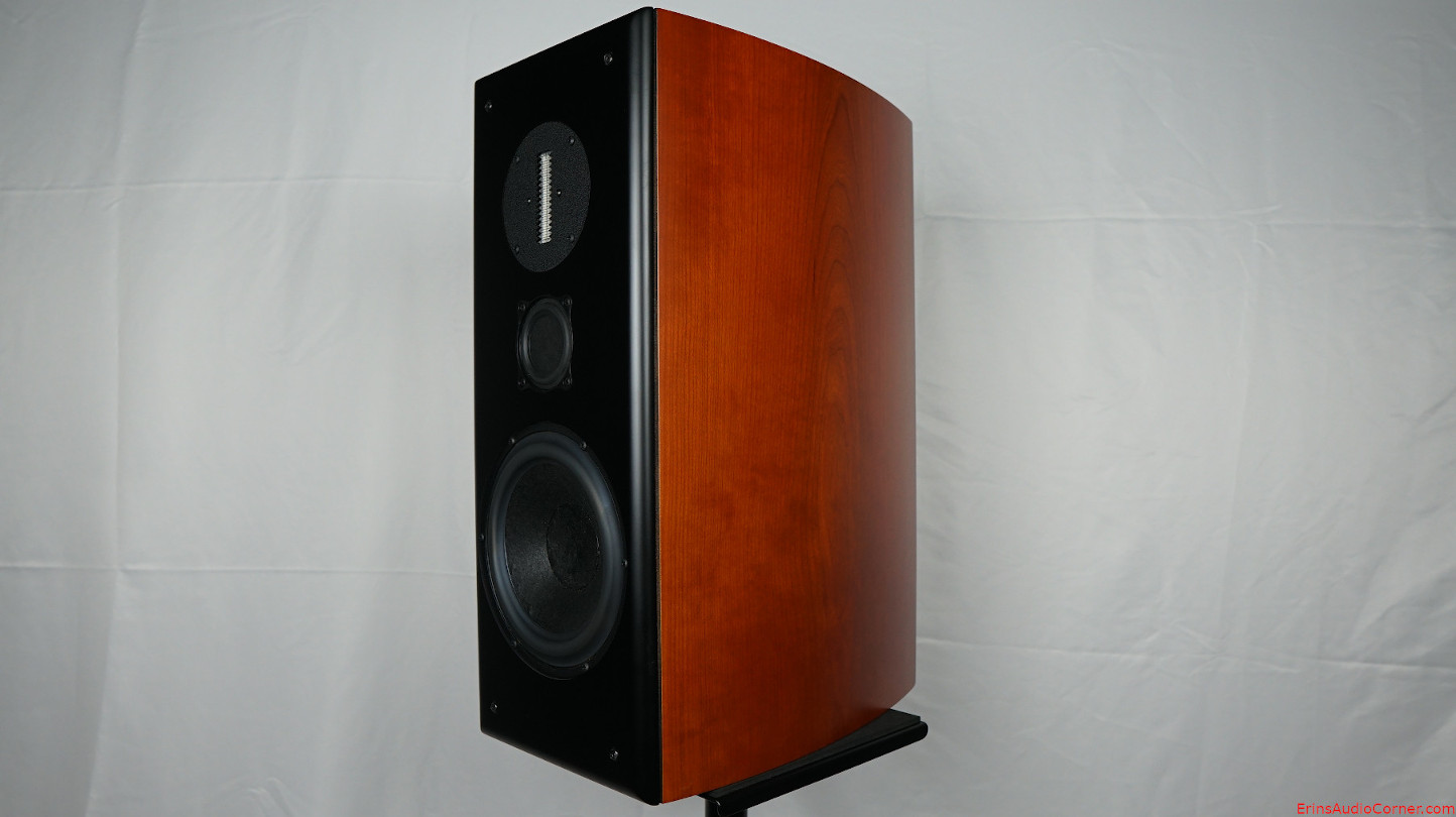
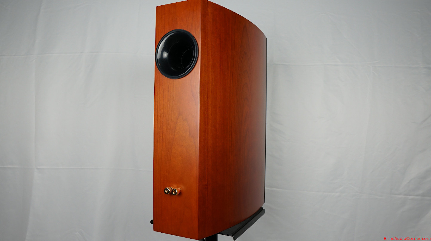
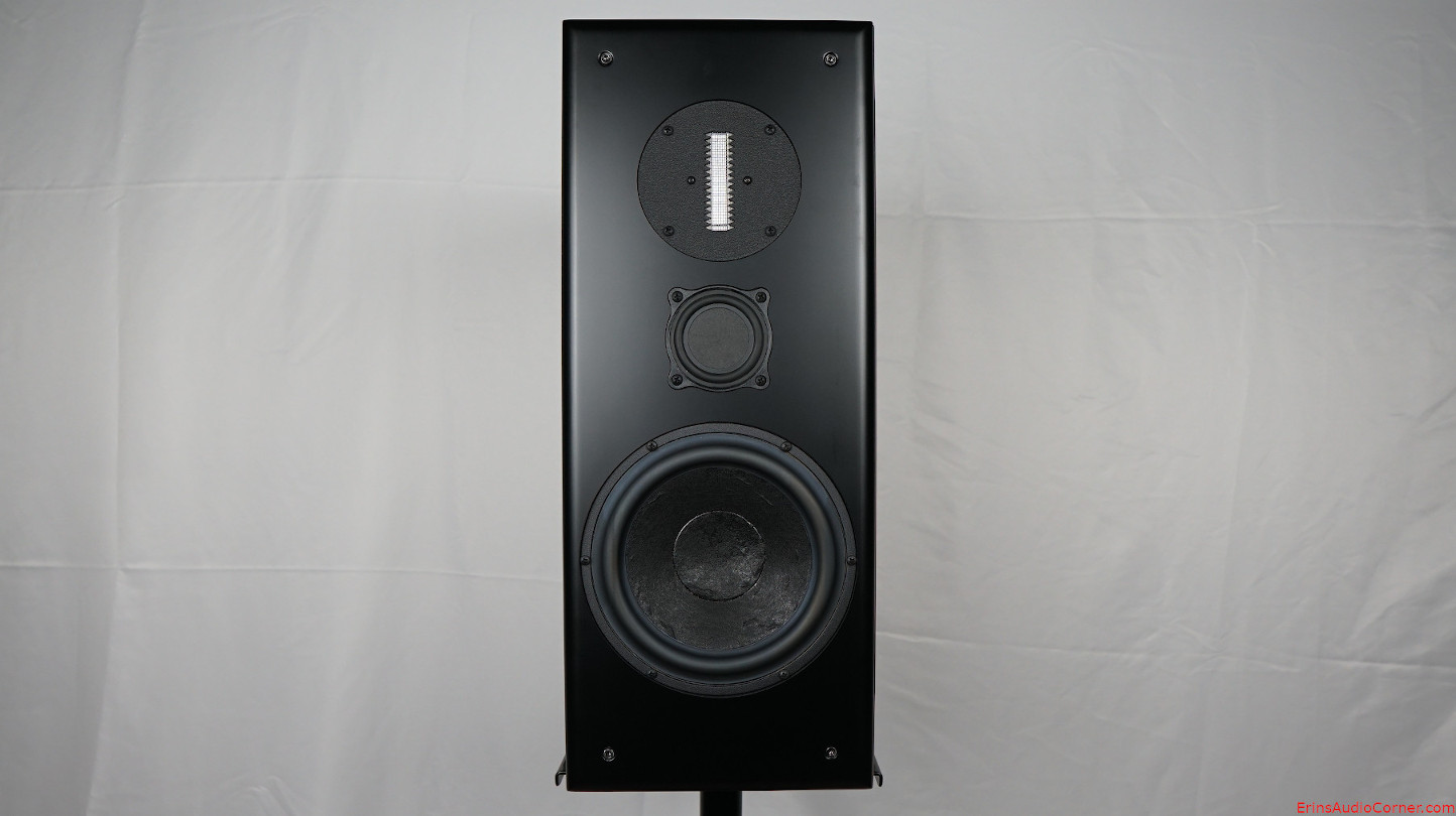
Dennis Murphy designed the Philharmonic BMR some years back and it lit up the DIY circuit. This is a 3-way “bookshelf” (a big bookshelf) incorporating the following drive units: RAAL, 64-10 Ribbon Tweeter, BMR 2.5″ Midrange, and Scan-Speak 18W8545-1 Paper-carbon cone woofer. There are countless threads about this speaker and the design available via a simple Google search so I won’t spend my time going on about it. It is important to note, though, this speaker tested is in a different cabinet than current offerings. This shouldn’t effect the results of the test considerably (I assume the same volume and port tuning is used with the various enclosure shapes) but it is worth noting as some response differences can arise with a rounded enclosure with a flat baffle vs other designs some may come up with for their own enclosure.

The speaker can be purchased complete through Salk Sound for $2395 - 2595, depending on what finish you purchase. Alternatively, this speaker can be built as a kit via Meniscus Audio and you can also even purchase a “flat-pack” for the cabinet from Speaker Hardware. Fully assembled (but unfinished), the DIY route would cost you in the neighborhood of $1150 to 1450 (depending on the flat pack order) and if you decided to upgrade components from Meniscus you could do so as well.

Foreword: Subjective Analysis vs Objective Data (click for more)

If you have seen my past reviews, you know that I am of the mindset that objective data is at least as important as someone's subjective evaluation of a speaker. If not more. Why? Because every room is different. Every listener is different. Some know what to listen for. Others know what they want to hear based on their own preference (i.e., some prefer extended bass, some prefer more midbass punch between 120-150Hz, some prefer a response with a dip around 4kHz, etc., etc.). What one person wants or expects may be opposite of another. Additionally, the room will impact the performance and therefore what the listener hears. This means when you read another's subjective-only review you are left to resolve those variables on your own. That's not likely to happen. Unless there is objective data you can use to get an idea of the performance. With objective data you can begin to understand why the subjective review turned out the way it did. Notably, objective data keeps reviewers honest. It's hard for a reviewer to legitimately bash one product but elevate another when the two measure practically the same in every regard. Not to say two similarly measuring speakers cannot subjectively sound different. Though, odds are if they do measure the same then a huge subjective difference is most likely attributed to other issues such as setup conditions, bias, etc. Objective data is the key to accountability. Simply put: if the measurements are taken with care and you understand them, you can rely on data to help paint a more accurate description of performance than a few adjectives from your favorite reviewer (myself included). As you will see, objective measurements can provide a lot of insight in to how the speaker will perform in your room.

However, when possible, it is always best to demo speakers in your own room. Not simply because of subjective performance. But because of other factors such as aesthetics, pride of ownership, etc. In my experience, all these factors play in to how the listener “connects” with the system. A good shop or manufacturer understands this and allows buyers to try items out at home before purchasing or they offer a reasonable return policy. If you question the performance and can demo the speakers in your own home, I suggest you take advantage of the opportunity.

For all the reasons listed above: What I provide here is objective-heavy analysis. I still provide my own subjective experience but with in-room measurements at my listening position(s) so we can understand why I heard what I heard. Is it the room, the actual speaker itself, my brain, or a combination?

Now that you understand my motives, let’s get started with the review.

Product Specs and Photos

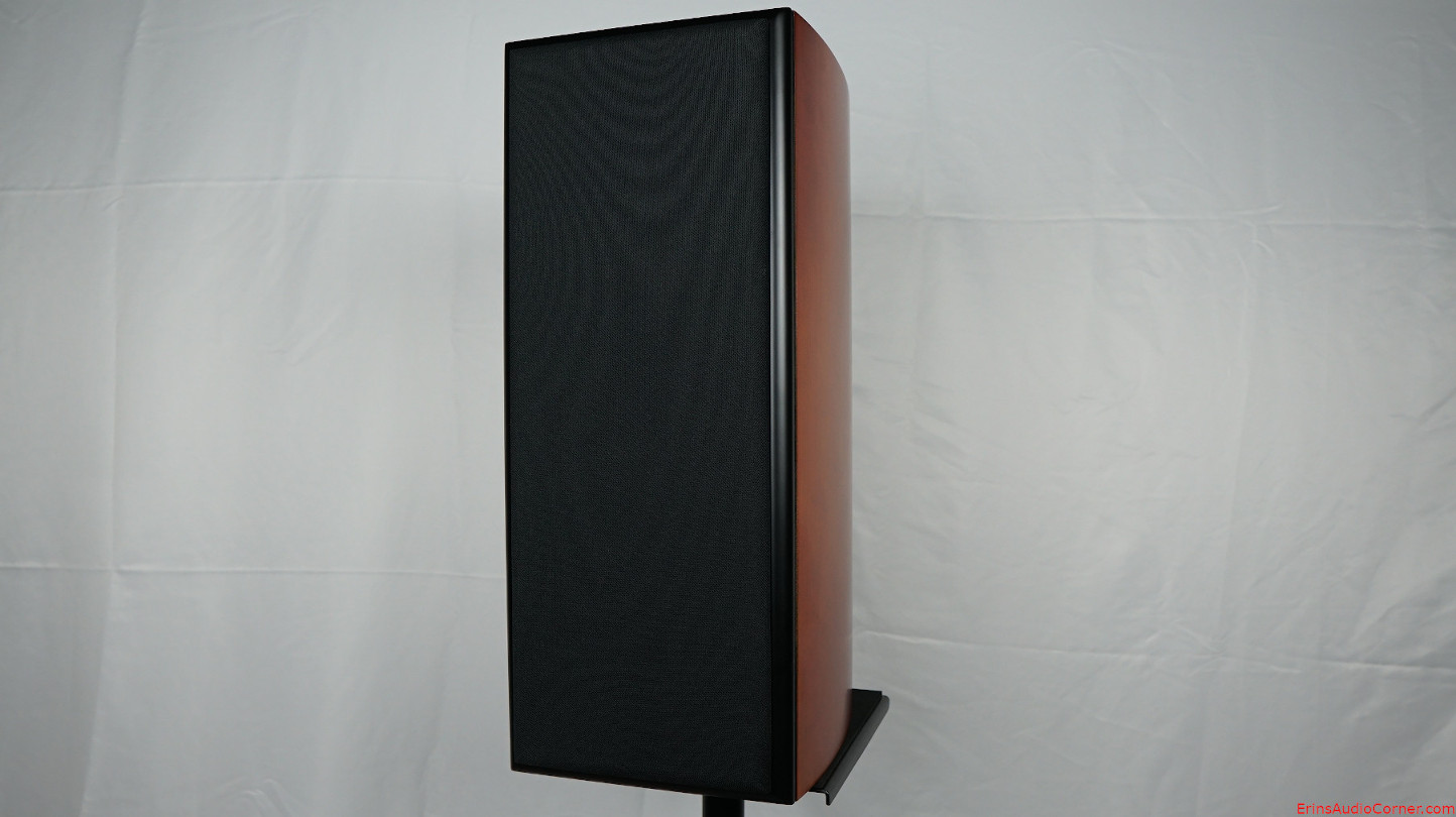
Grille On:

Objective Data

Unless otherwise noted, all the data below was captured using Klippel Distortion Analyzer 2 and Klippel modules (TRF, DIS, LPM, ISC to name a few). Most of the data was exported to a text file and then graphed using my own MATLAB scripts in order to present the data in a specific way I prefer. However, some is given using Klippel’s graphing.

Impedance Phase and Magnitude:

Impedance measurements are provided both at 0.10 volts RMS and 2.83 volts RMS. The low-level voltage version is standard because it ensures the speaker/driver is in linear operating range. The higher voltage is to see what happens when the output voltage is increased to the 2.83vRMS speaker sensitivity test.

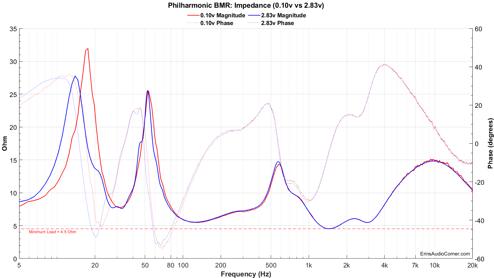
From the above data we can see the following:

The tuning frequency of the enclosure is approximately 32Hz.
The minimum impedance dips to about 4.5 Ohms around 1.4kHz with a nominal impedance at 6 Ohms. You might be able to power this with a standard AVR (as long as it is 6 Ohm rated). However, the low sensitivity of this speaker and a long listening distance means it will need ample power to get to higher output levels so choose how you power this speaker accordingly.
There are no signs of resonance (typically visible as bumps/wiggles in the impedance that deviate from the curve).

Frequency Response:

Notes about measurements (click for info)

Frequency response data (horizontal, vertical, “Spinorama”, polar, spectrograms, etc.) are all based on a 2.83 volts RMS logarithmic sweep at 1 meter to meet the standard sensitivity measurement spec. These data are captured using Klippel’s TRF module and a mixture of ground-plane measurement and 4-pi free-field measurement. Klippel’s In-Situ Room Compensation (ISC) module is then used with the ground plane measurement to provide a ‘reference’ curve to the 4-pi measurement which then corrects for the room’s influence and allows me to generate a reflection-free far-field response from an indoors measurement. Note: This is not a standard merge of nearfield and farfield nor a merge of ground-plane and farfield. Typical merged responses still suffer low resolution in the midrange where the response is merged due to the necessity of windowing the impulse response to remove reflections. One major downside to “gating” or “windowing” the impulse response is this low-resolution does not show resonance in the midrange. For example, most free-field measurements are only reflection-free until approximately 3 milliseconds, or about 300Hz. That means a data point every 300Hz. If you have a high-Q resonance at 450Hz the 300Hz resolution data will not show this resonance because the frequency resolution only has a data point at 300Hz and 600Hz; skipping right over the 450Hz. You would need a resolution of at least a half the width of the Q-factor; generally, 20Hz is adequate. However, 20Hz resolution is roughly 50ms of window-free response. The only way to achieve this is in a large parking lot or open field. Ground plane measurements are perfect for this but are subject to aiming/ground absorption (grass) and related issues above 400Hz. The ISC module permits results with as-close-to-anechoic as one can achieve without being anechoic. Thanks to the ISC module, the data I am providing here is higher resolution (~30Hz resolution) than an average person can provide without access to an anechoic chamber or the like.

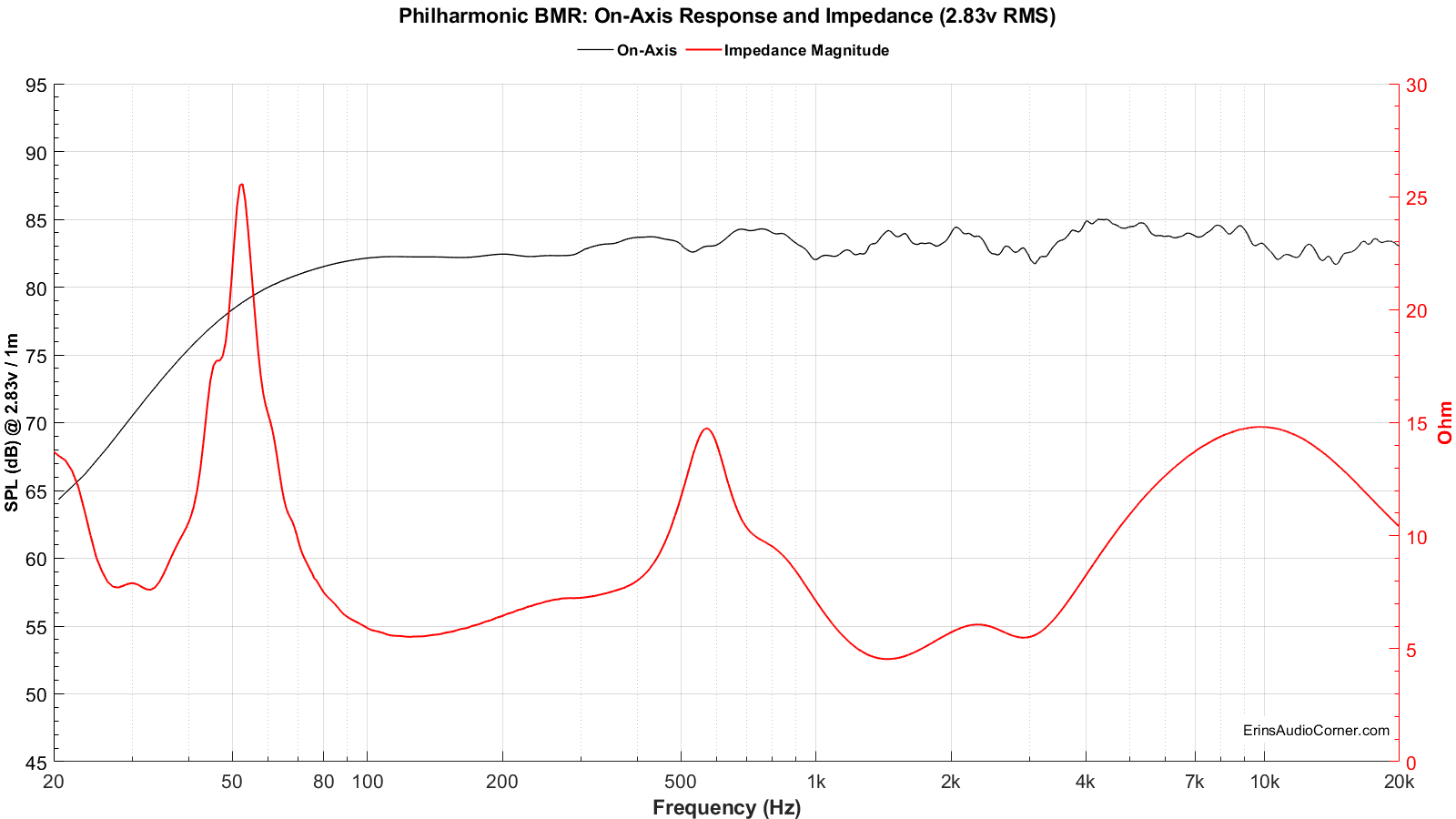
The measurement below provides the frequency response at the reference measurement axis - also known as the 0-degree axis or “on axis” plane - in this measurement condition was situated at the ribbon.

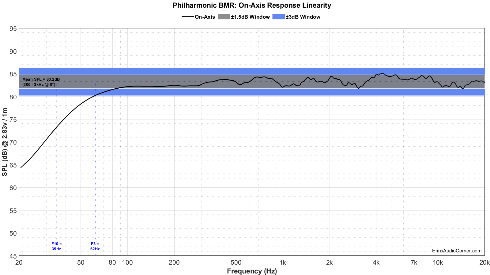
The mean SPL, approximately 83.2dB at 2.83v/1m, is calculated over the frequency range of 300Hz to 3,000Hz.

The blue shaded area represents the ±3dB response window from my calculated mean SPL value. As you can see in the blue window above, the Philharmonic BMR has a ±3dB response from 62Hz - 20kHz. Even better, a tighter window of linearity is provided in gray as ±1.5dB from the mean SPL and this speaker stays within this window from about 80Hz all the way to 20kHz (ignoring the 0.1dB around 4kHz). That is impressive!

The speaker’s F3 point (the frequency at which the response has fallen 3dB relative to the mean SPL) is 62Hz and the F10 (the frequency at which the response has fallen by 10dB relative to the mean SPL) is 35Hz. This speaker has nice low frequency extension.

The one thing I find a bit odd is the 1dB shelf below 300Hz. I can’t imagine this being baffle step because, from what I can tell, the crossover point between the woofer and the midrange is about 550Hz.

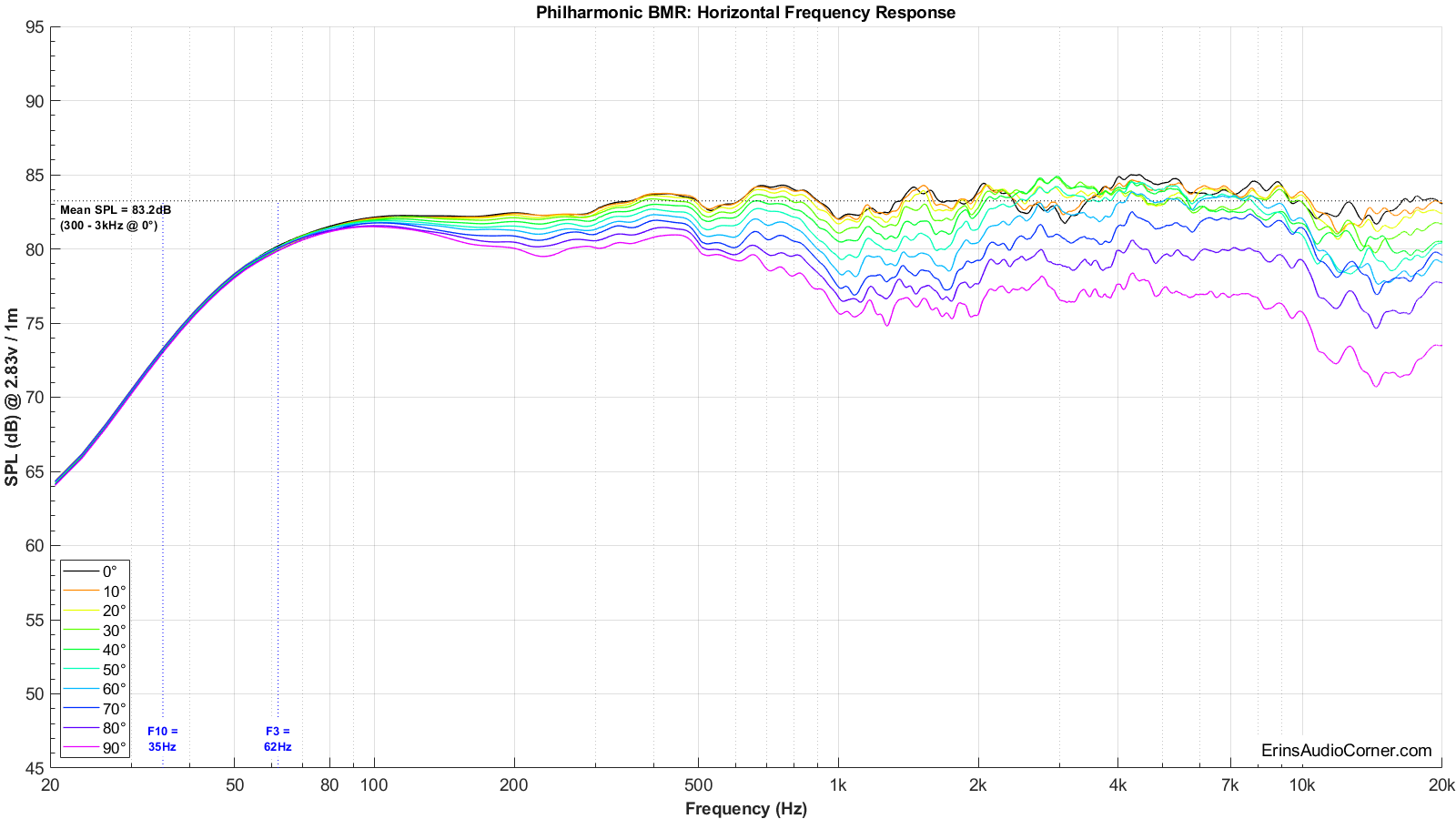
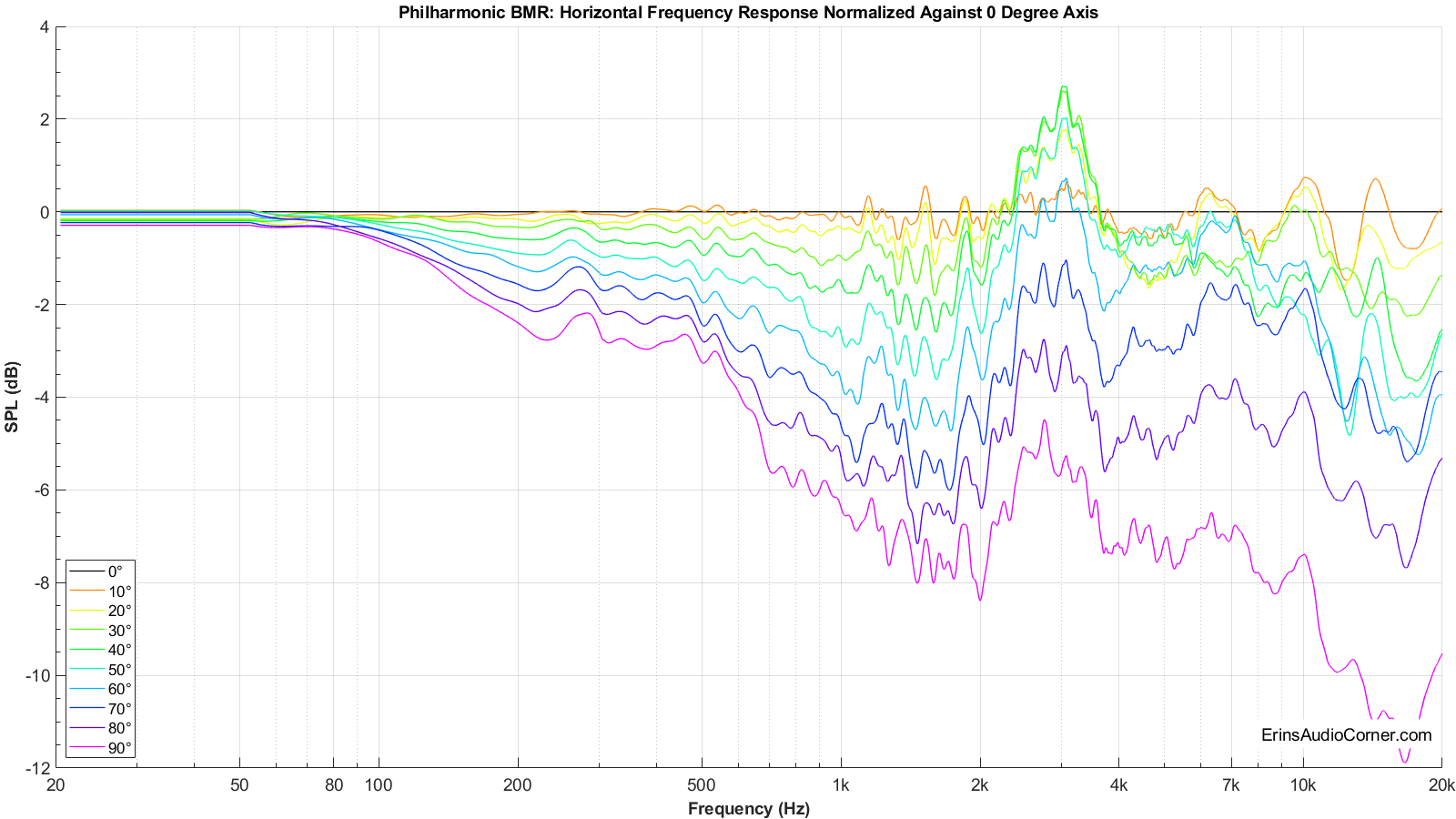
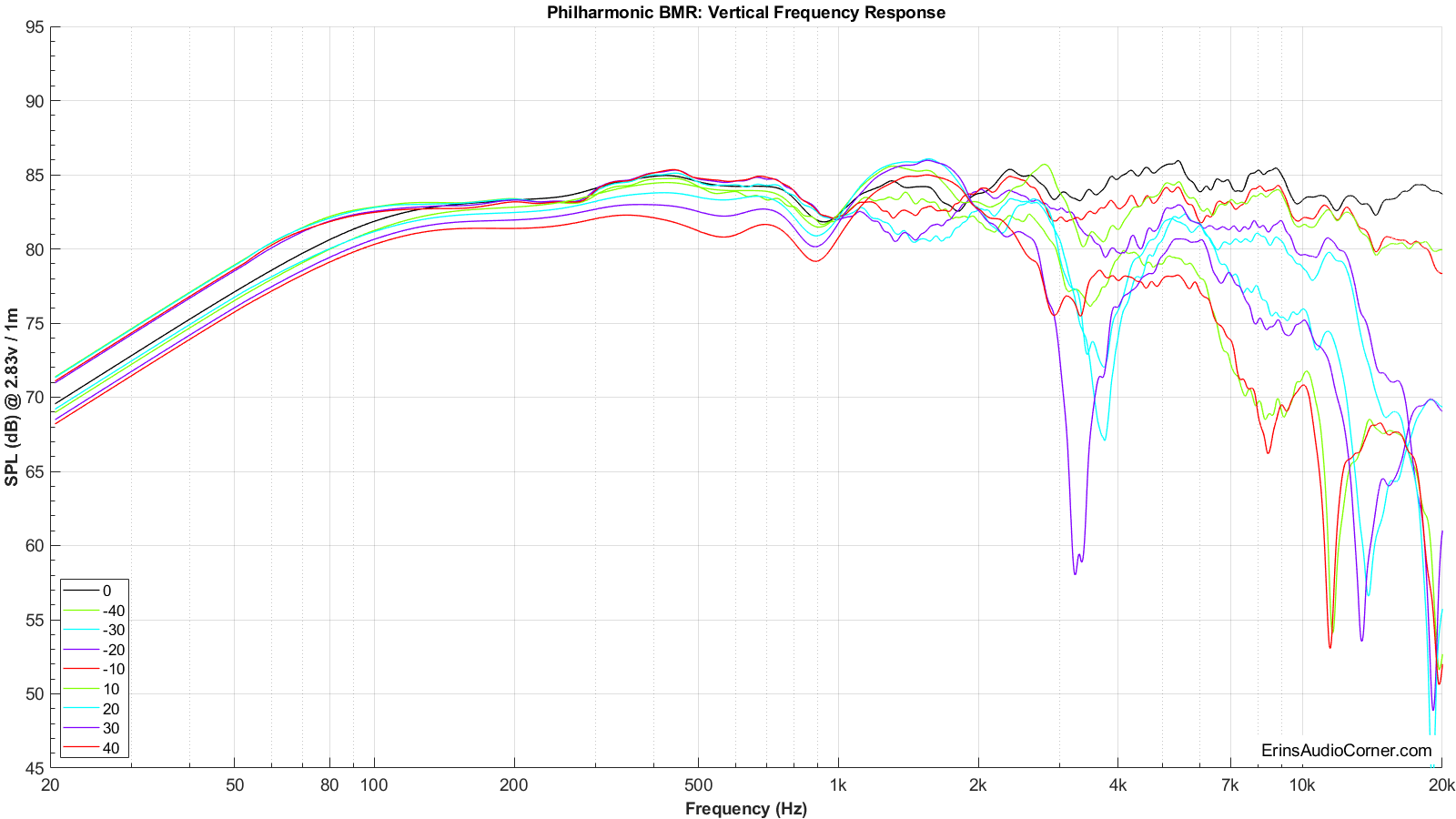
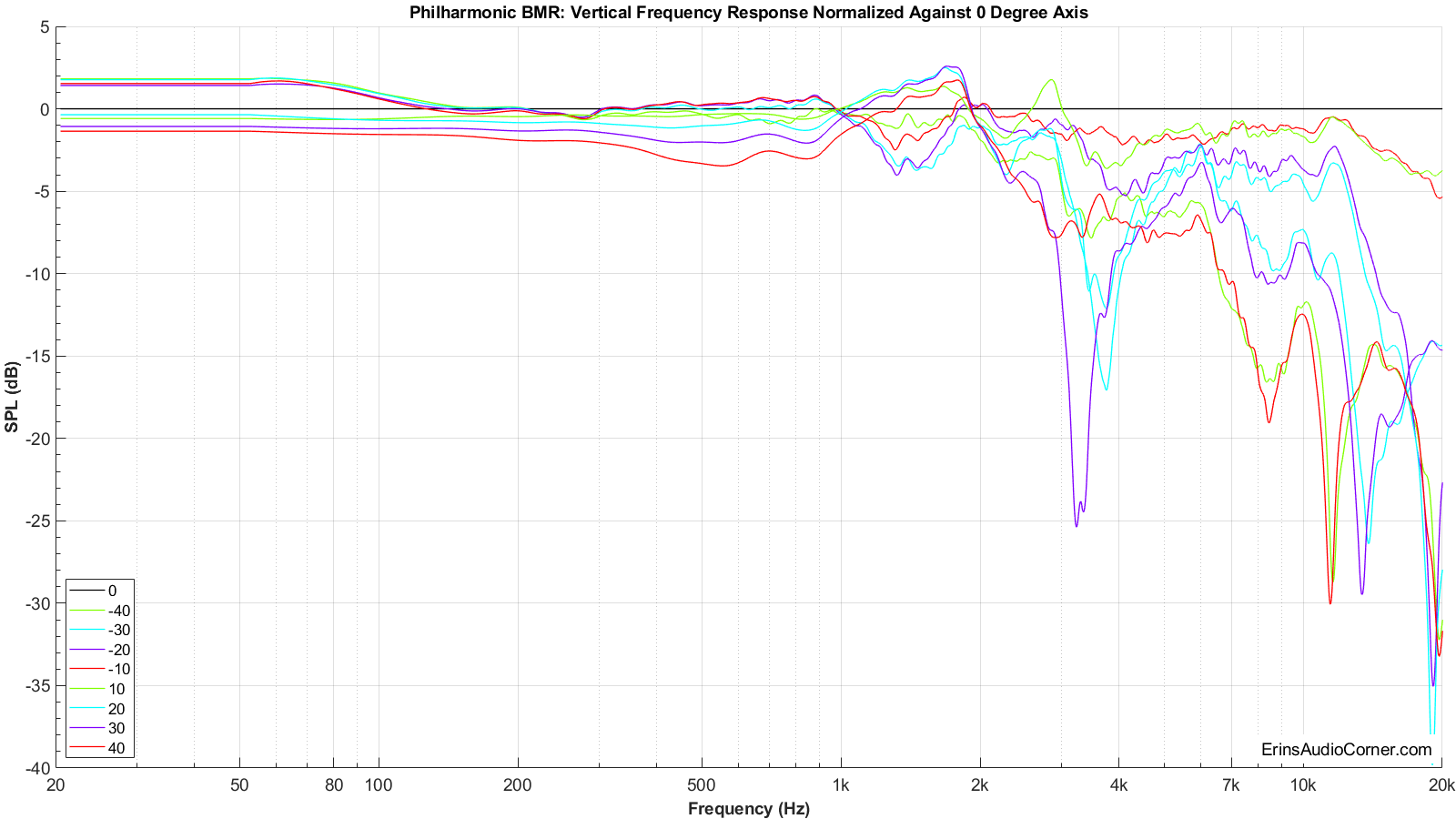
Below are both the horizontal and vertical response over a limited window (90° horizontal, ±40° vertical). I have provided a “normalized” set of data as well. The normalization simply means that I took the difference of the on-axis response and compared the other axes’ measurements to the on-axis response which gives the viewer a good idea of the speaker performance, relative to the on-axis response, as you move off-axis.

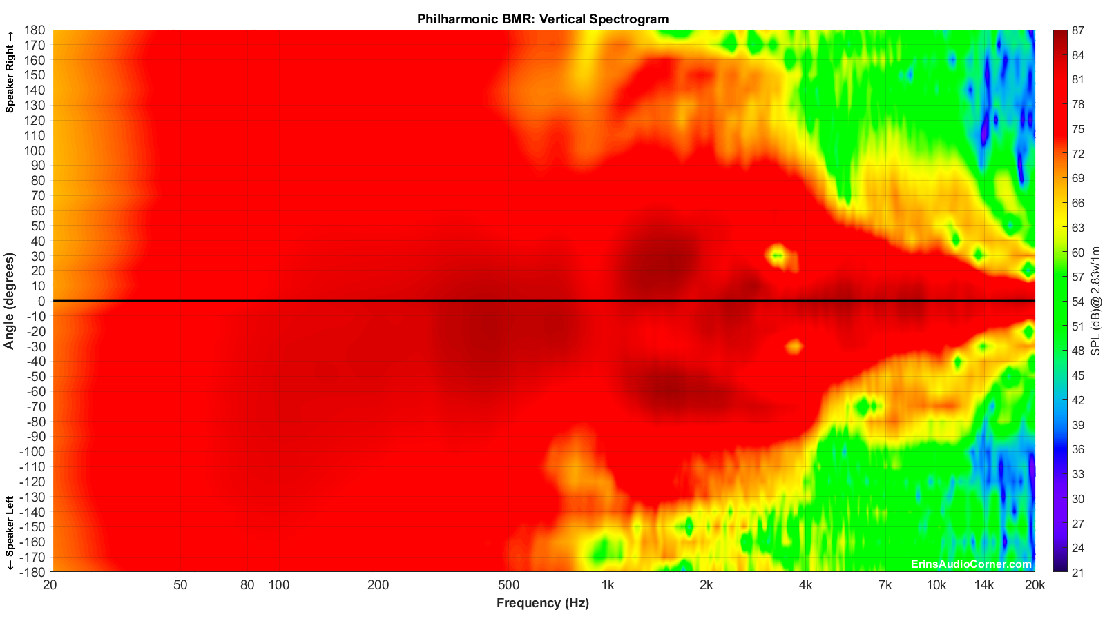
As I said above, the provided frequency response graphs were given with a limited set of data. I measured the response of the speaker’s vertical and horizontal axis in 10-degree steps over 360-degrees. Nearly 70 measurements in total are represented in my data. As you can imagine, providing all those data points in a single FR-type graphic below is a bit overwhelming and confusing for the viewer. A spectrogram is an alternate way to view this full set of data. This takes a 360-degree set of data and “collapses” it down to a rectangular representation of the various angles’ SPL. I have provided two sets of data: one set for horizontal and one for vertical. Each set consists of 2 graphics:

Full response (20Hz - 20kHz with the angles from 0° to ±180°) with absolute SPL values
Full, “normalized” response (20Hz - 20kHz with the angles from 0° to ±180°) with SPL values relative to the 0-degree axis

Normalized plots make it easier to compare how the speaker’s off-axis response behaves relative to the on-axis response curve.

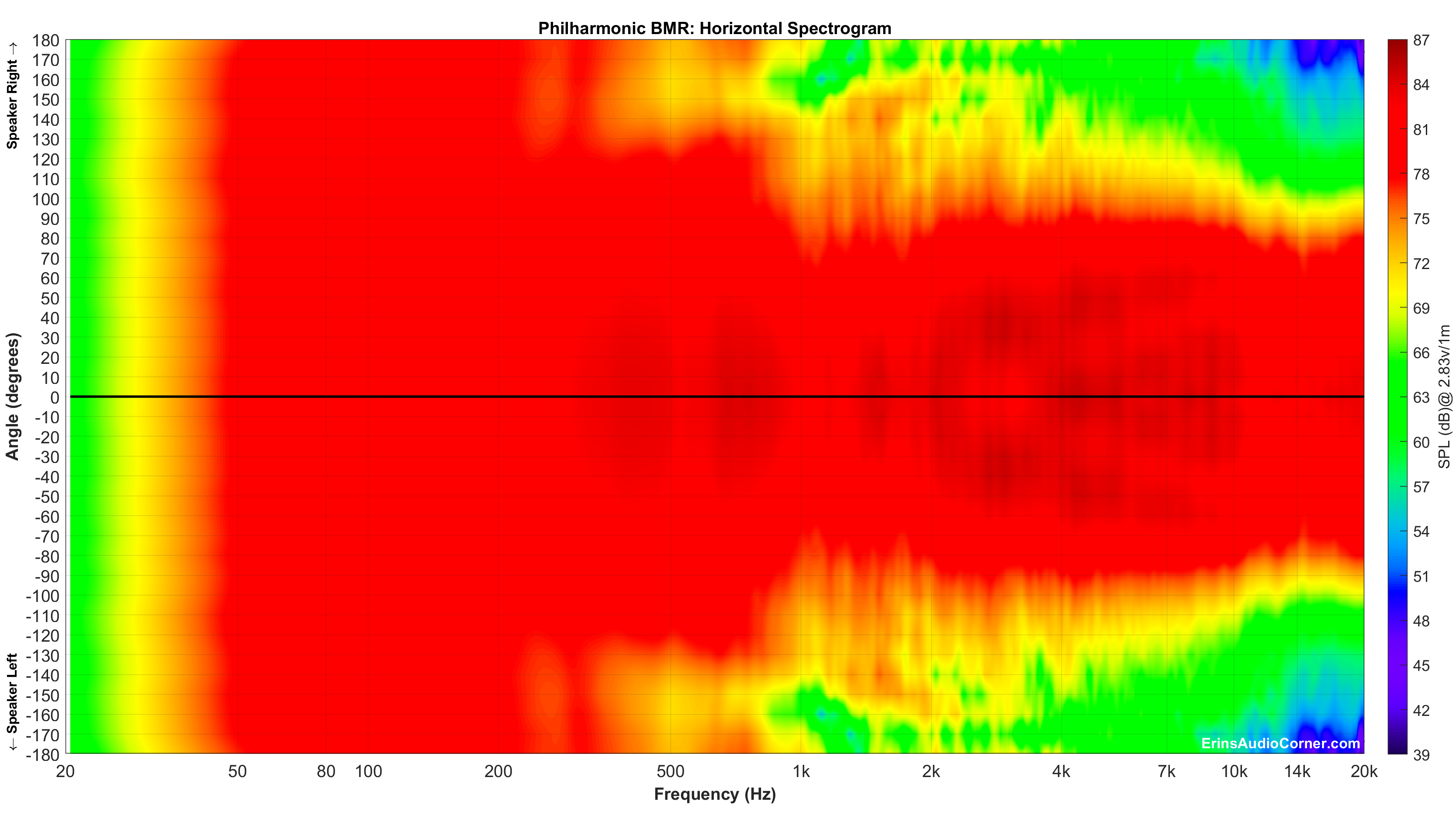
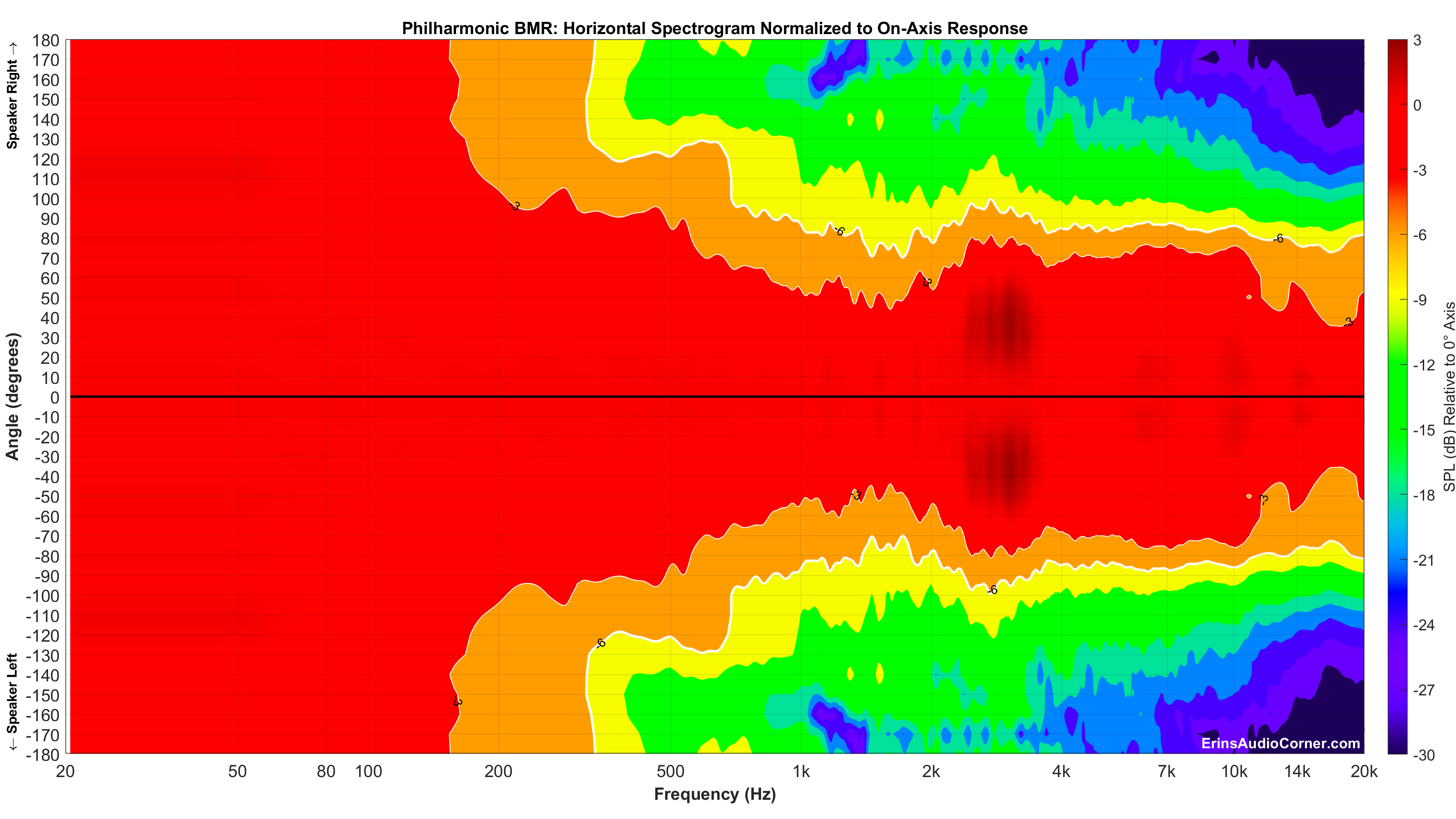
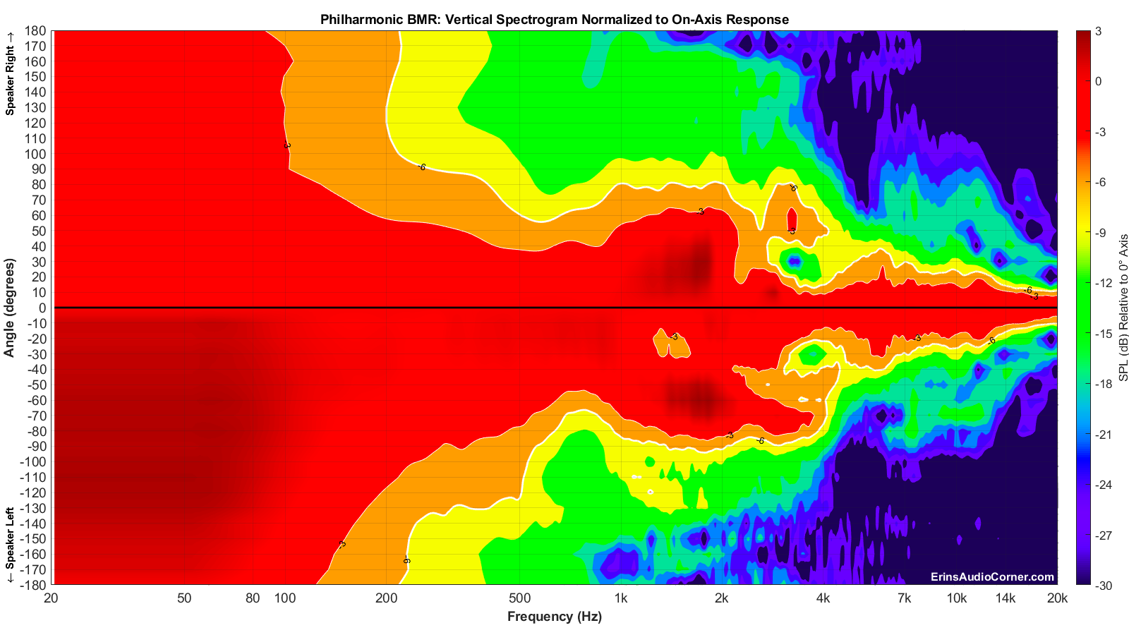
The above spectrograms are the standard way of providing directivity graphics by most reviewers. Some prefer not to normalize the data. Some prefer to normalize the data. Either way, it’s a useful visual to get an idea of the directivity characteristics of a speaker or driver.

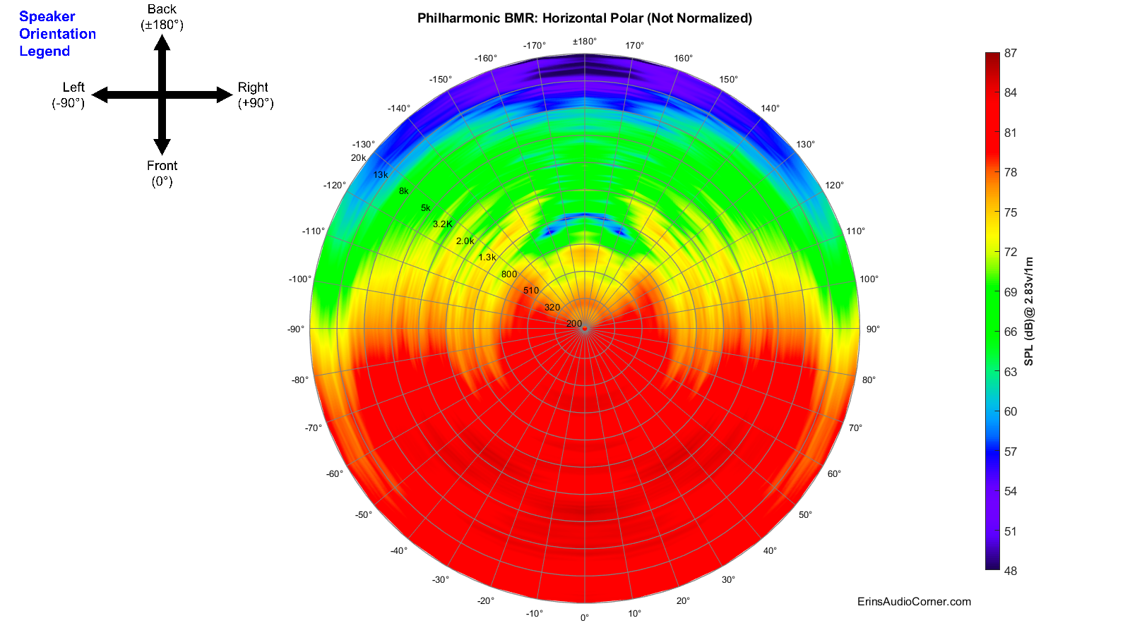
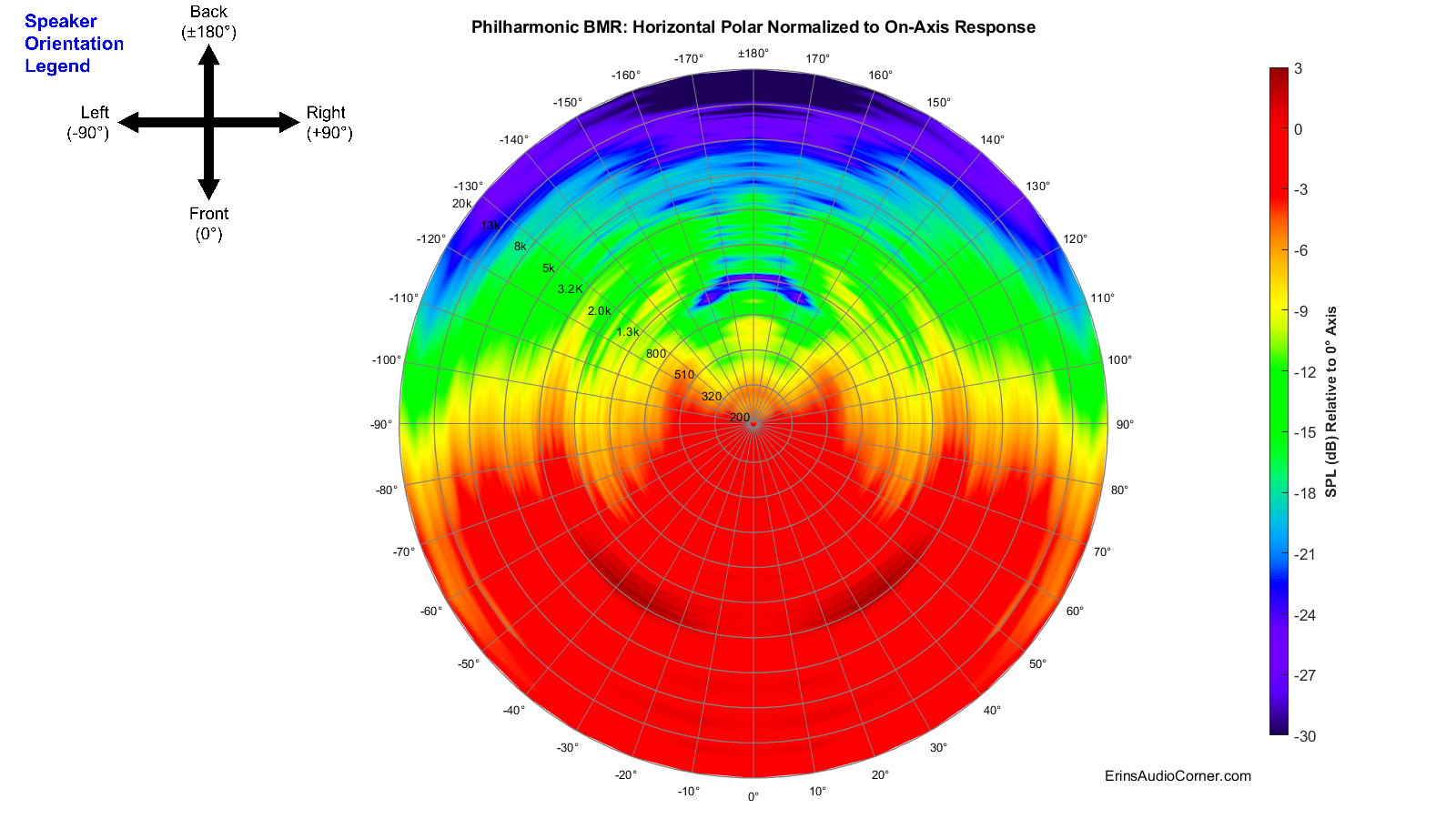
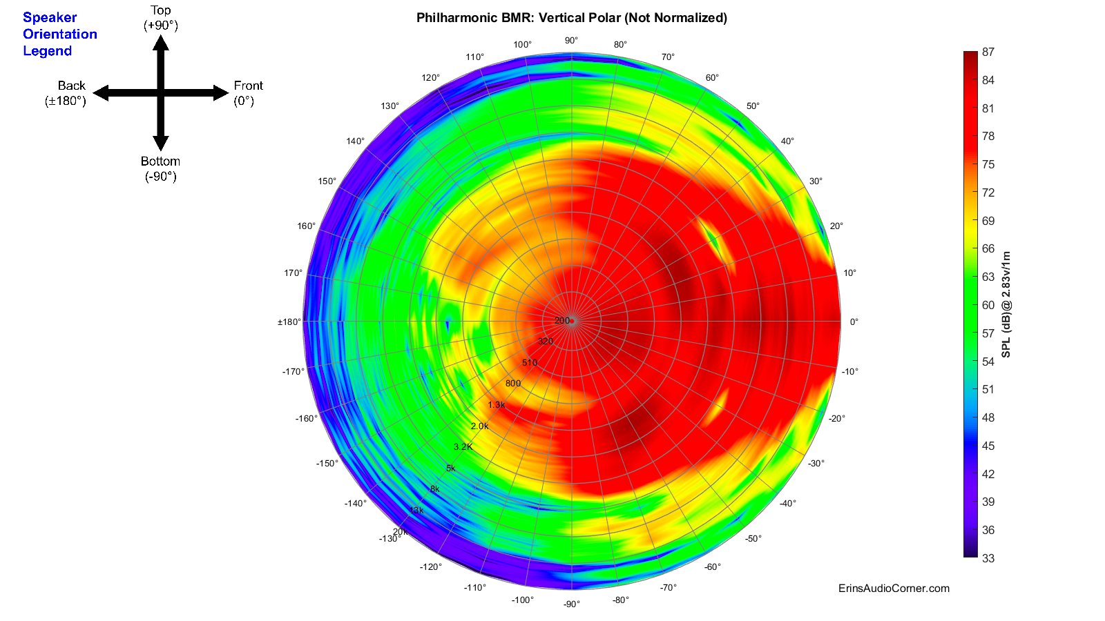
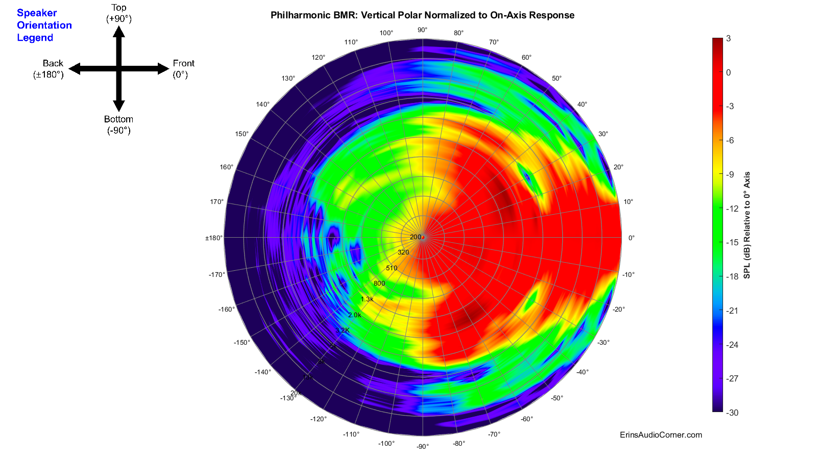
However, these “collapsed” representations of the sound field are not very intuitively viewed. At least not to me. So, I came up with a different way to view the speaker’s horizontal and vertical sound field by providing it across a 360° range in a globe plot below. I have provided both an absolute SPL version as well as a normalized version of both the horizontal and vertical sound fields.

Note the legend provided in the top left of each image which helps you understand speaker orientation provided in my global plots below.

CEA-2034 (aka: Spinorama):

The following set of data is populated via 360-degree, 10° stepped, “spins” from vertical and horizontal planes resulting in 70 unique measurements. Thus, this is sometimes referred to as “Spinorama” data. Audioholics has a great writeup on what these data mean (link here) and there is no sense in me trying to re-invent the wheel so I will reference you to them for further discussion. However, I will explain these curves lightly and provide my own spin on what they mean (pun totally intended). Sausalito Audio also has a good write-up on these curves here. Furthermore, you can find discussion in Dr. Floyd Toole’s book “Sound Reproduction”. Here’s my Amazon affiliate link if you want to purchase it and help me earn about 2% of the price. And, finally, here is a great video of Dr. Toole discussing the use of measurements to quantify in-room performance.

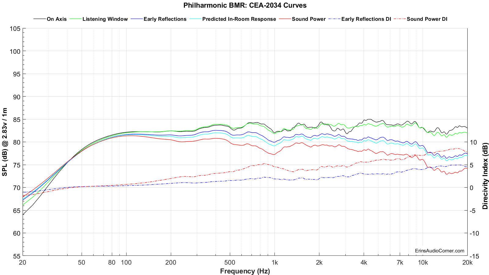
In short, the CEA-2034 graphic below takes all the response measurements (horizontal and vertical) and applies weighting and averaging to sub-sets and can help provide an (accurate) prediction of the response in a typical room. If there is a single set of data to use in your purchase decision, this is probably it.

Alternatively, click this arrow, if you want my quick take on what these curves mean without going to another site.

On-Axis is simply the on-axis response. This is the 0-degree response curve.
Listening Window is an average of the 0° to ±30° horizontal and 0° to ±10° vertical response curves and is used to understand what listeners typically hear in a home at the sweet spot, or Main Listening Position (MLP). The reason for this extended window of sound is simply because your room makeup might differ from another’s. This curve is an attempt to quantify a speaker’s performance over a smaller window that is often the norm for listening angle differences in various homes. It is important for this curve to very closely mimic the on-axis response. Deviations of the Listening Window curve relative to the on-axis response curve indicates a compromise in the speaker; often caused by directivity changes (as a speaker transitions from one drive-unit to another a la midwoofer to tweeter, or as a tweeter’s response becomes highly directional).
Early Reflections is very useful because it helps us determine how the room’s influence will alter (corrupt, most of the time) the direct (on-axis) response. Ideally, the speaker radiates sound uniformly with no aberrations; no resonance, no directivity changes as the speaker transitions from the mid to the tweeter and so on. Because speakers often have these issues, however, what is reflected to us from the walls, ceiling and floor is not the same as what we hear from the on-axis, direct sound. And that’s a problem. Why is that a problem? As stated in Dr. Toole’s book “these are very influential in establishing timbral and spatial qualities”. Large deviations in this relative to the on-axis response also indicate areas where the room is of consequence. Also, it is important to understand the Early Reflections response is made up of rear-firing sounds. A speaker drive-unit is omnidirectional (radiating in all angles evenly) until the half-wavelength equals that of the drive-unit diameter. When the diameter is larger than the wavelength being played, the sound transitions from omnidirectional to directional; also known as “beaming”. Even tweeters beam. For example, a 1-inch dome tweeter will beam at approximately 6750Hz (speed of sound ÷ 2 ÷ diameter). In most speakers you have a single tweeter, firing forward. You can imagine that the high-frequency response in the front of the speaker would therefore be quite different than what is measured behind the speaker. So, being that the Early Reflections curve includes rear-hemisphere measurements you can understand that the high-frequency response would slope downward vs the on-axis response. This is understood and accepted.
Predicted In-Room Response curve has the benefit of showing directivity mismatches at the crossover as well as resonances easily by comparing them to the overlaid Target curve (further down).
Directivity Index (DI) curves are the difference in the Listening Window and the respective Early Reflections or Sound Power curves. My understanding, currently, is the Sound Power and Sound Power DI aren’t quite as useful for typical homes. However, there is emphasis placed on the Early Reflections DI curve. The right Y-Axis provides a value associated with the DI curves. The higher the number, the more directional the speaker. For example: a “0” DI curve - a curve which is completely flat - would be a speaker that is purely omnidirectional; radiating uniformly in all angles vertically and horizontally. A speaker that increases over frequency means that it is radiating in a tighter window as you increase in frequency. This is typical because, as I discussed above, even tweeters beam… and most speakers have a single tweeter facing the front and therefore, the speaker becomes directional at whatever the tweeter’s beaming frequency is. There isn’t necessarily a one-size-fits-all DI curve value. Though, it seems people (myself included) prefer a speaker with a wider soundstage which is found in lower directivity speakers (because more sound is bouncing off the side walls; which confuses the use of side-wall absorption but that’s for a later debate). However, what is important is that the curve, however tall you may prefer it to be, is smooth; almost linear. Dips and peaks mean that something, not good, is going on. But a linear curve indicates excellent transition through crossover regions, no resonance, etc. Since speakers are not perfect, though, linear DI curves are not the norm. Speakers become directional as they increase in frequency, around strong resonances, and as the sound transitions at the crossover from one drive-unit to another and you wind up with areas with peaks and/or dips whether they’re spread through a wide frequency range (low-Q) or very sharp/drastic (high-Q). But when you’re looking at the Early Reflections DI curve, look for this: smooth.

The following are my takeaways from the data. More may be obvious to others or myself (with more time).

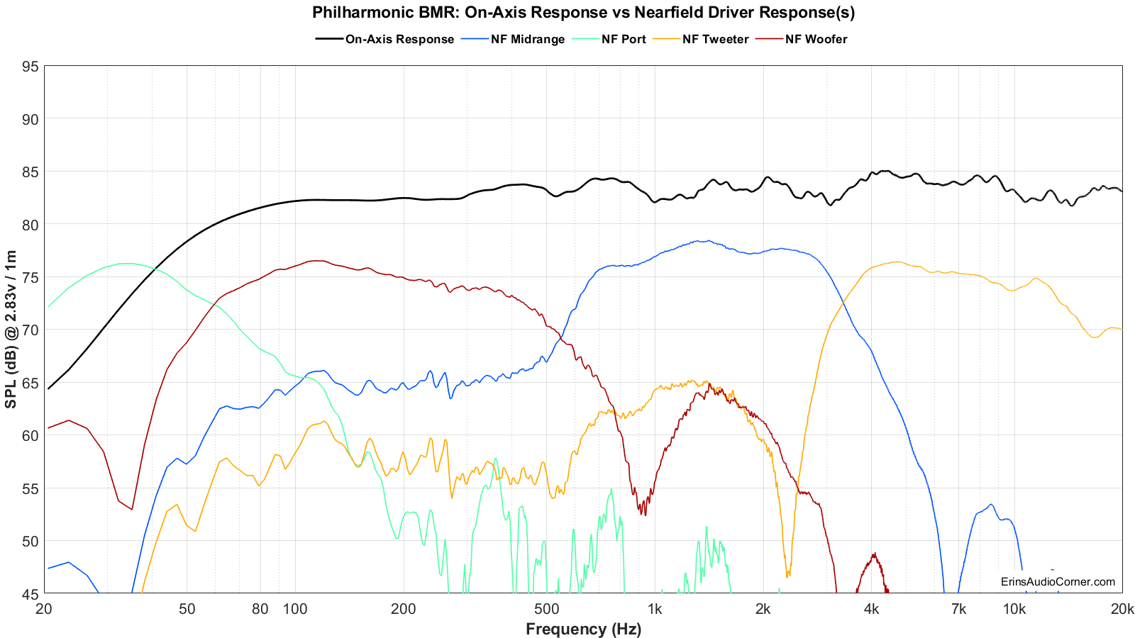
There are various ways you can interpret the data, substituting the “dips” for “peaks” in analysis of the non-linearity. For example, I see the 400-500Hz and 700-800Hz regions as potential resonances (namely, the latter). However, if you view the 500Hz and 1kHz regions as dips, then one could argue the other bumps in response are not resonances. Looking at the nearfield data (in the Miscellaneous section), it appears the woofer has a notch at approximately 1kHz. I pulled up the driver data for the Scan-Speak 18W8545-1 and see there is a 2dB tall resonance spread from about 600-700Hz so I’m inclined to believe this really is a resonance, but not breakup, albeit small. Without disabling the other drive-units, however, it is hard to know for sure.
The Listening Window lies mostly within the on-axis response but notably different at ~2.5kHz to 3.1kHz. This is within the region of the crossover between the midrange and the tweeter. You’ll notice in the above graphics that the off-axis response of the horizontal response yields a bump in this region compared to the on-axis response. Additionally, the RAAL is quite directional, vertically, due to its tall orientation. Therefore, it “beams” at approximately the frequency that equals the radiating height (70mm; 2.75 inches). Using the speed of sound and half-wavelength you can calculate the beaming point for this dimension as ~2.5kHz (SoS = 13500 under standard conditions: SoS/2/2.75 = 2449 Hz). So, the difference in the Listening Window vs the on-axis response is mostly caused by the horizontal response but the vertical directivity mismatch of the BMR midrange to the RAAL tweeter is a contributor as well.
Outside of the two comments above, this speaker displays a very nice set of CEA-2034 curves with relatively wide directivity index curves. It has very wide horizontal directivity (which can be observed in the spectrogram and global plots presented earlier) with a horizontal response window of ±60° (non-normalized) up to about 10kHz. However, the vertical directivity is considerably narrower thanks to the RAAL tweeter’s height as mentioned above. The vertical window begins to narrow considerably above about 4kHz where the tweeter is the provider of response.

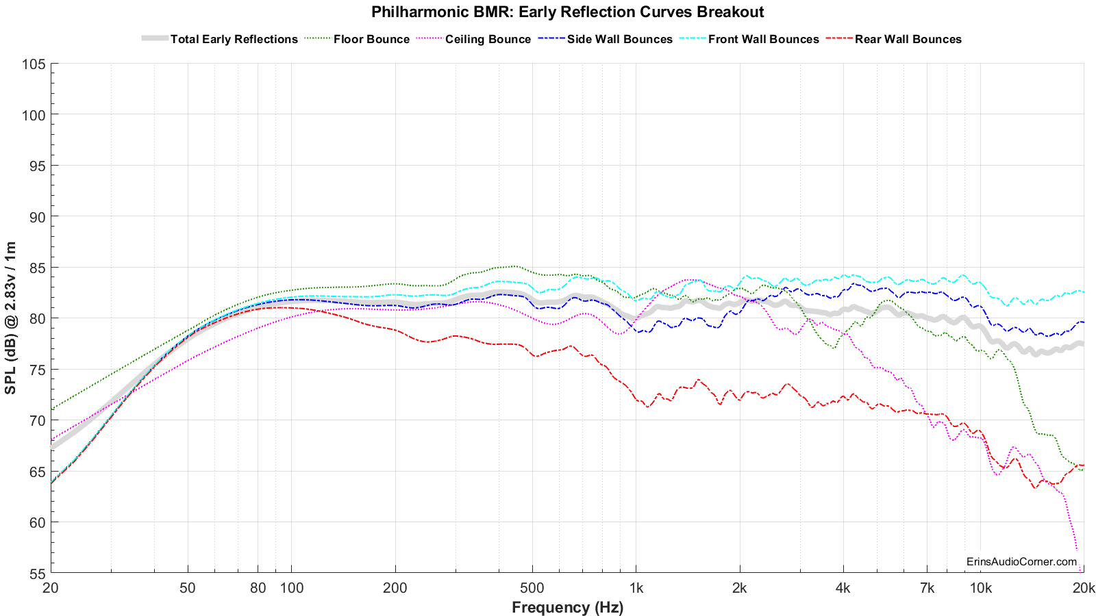
Below is a breakout of the typical room’s Early Reflections contributors (floor bounce, ceiling, rear wall, front wall and side wall reflections). From this you can determine how much absorption you need and where to place it to help remedy strong dips from the reflection(s). Again, as a pointer to the wide horizontal envelope, notice how the Rear Wall Bounces Curve is relatively high in amplitude (for a front-facing tweeter, at least) until about 10kHz.

And below is the Predicted In-Room response compared to a general Target curve equaling -1dB/octave. The -1dB shelf below 300Hz effects the location of this target curve. Additionally, this, speaker didn’t sound as bright as this overlay may indicate. Though, I did find it to be about 1dB too high in treble up until 10kHz where I wanted more “air”. The combination of what I heard and this shelf would probably put the target and predicted curves more in line with what I heard. Also, the Predicted In-Room response is a function of radiation. This speaker’s tweeter does not radiate like a typical dome tweeter and therefore has a much broader horizontal dispersion pattern, which seemingly causes the Predicted In-Room high frequency response to be more flat.

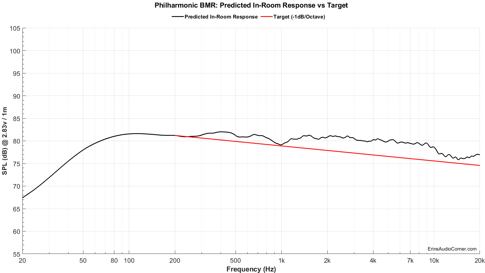
You may ask just how useful the above prediction is. Well, I’d be remiss for not delving in to that a little bit here. Please see my Analysis section below for discussion on this. :)

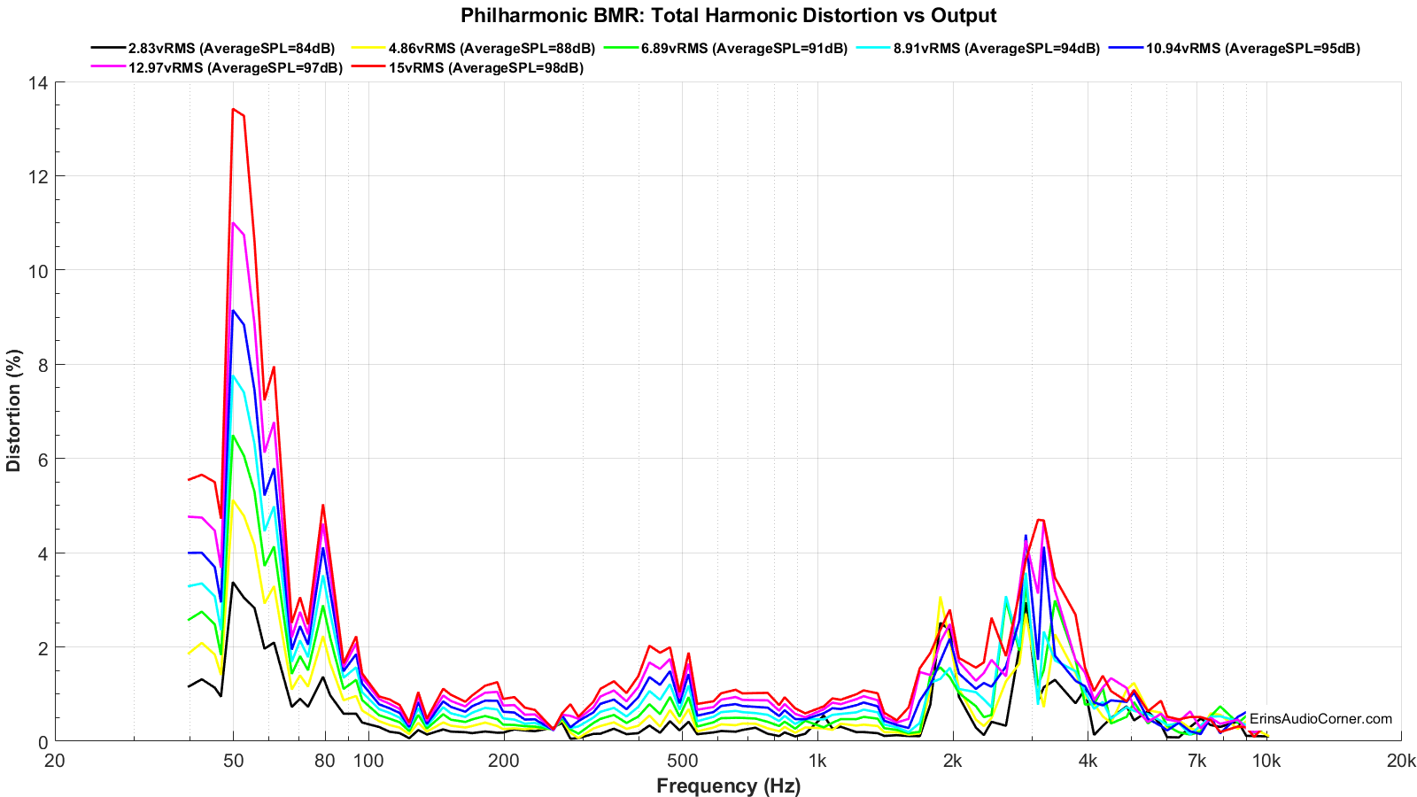
Total Harmonic Distortion (THD) and Compression:

Distortion and Compression measurements were completed in the nearfield (approximately 0.3 meters). However, SPL provided is relative to 1 meter distance.

Harmonic Distortion and Compression: What does this data mean? (click me for info)

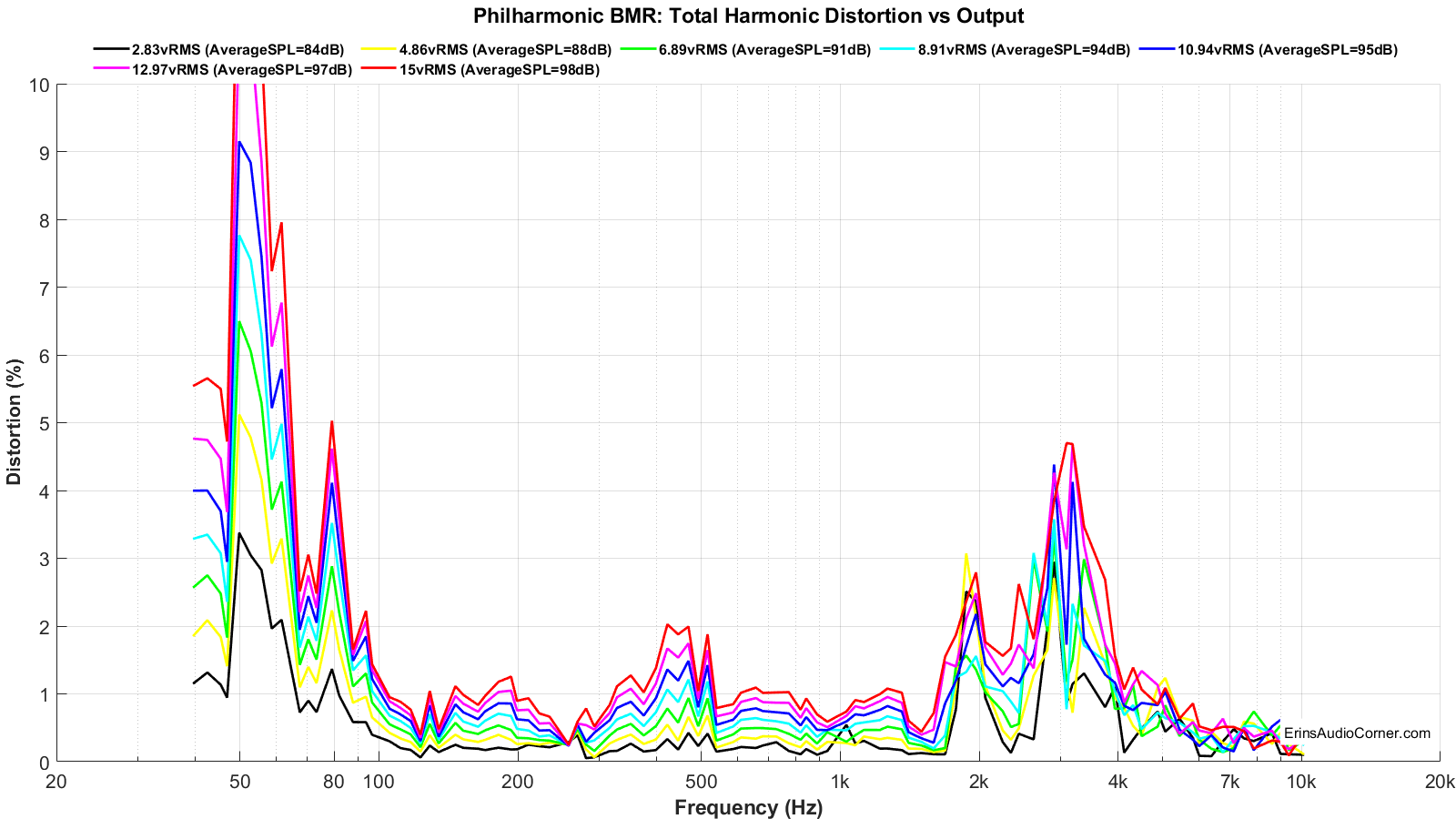
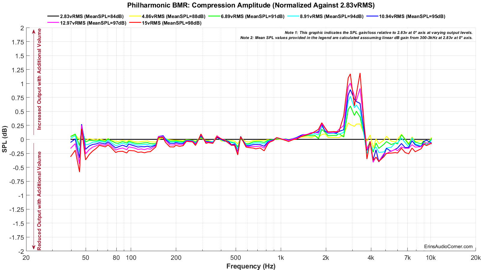
Harmonic Distortion and Compression are provided at varying levels to get an idea of what happens as the voltage into the speaker is increased and overall output volume increases. The “mean spl” values associated with each voltage provided in the legend is based on a calculation of expected volume assuming linear volume at the 300-3kHz region. Meaning, if a speaker is ideal and you tell your stereo to increase by 6dB by turning the volume knob +6dB, the output will increase by 6dB. In the real-world, however, a speaker is a mechanical device and there are compression effects that can limit the output volume and, therefore, you could possibly only get an actual increase in volume of 5dB. A good speaker will have little compression (< 1dB), where poorer speakers may suffer greater compression (> 2dB). Generally speaking, higher sensitivity speakers (like pro-audio speakers with 100dBSPL @ 2.83v/1m spec) suffer relatively no compression while lower sensitivity speakers (low 80’s dBSPL @ 2.83v/1m) suffer more compression. When a crossover is used the compression near the speaker’s Fs is attenuated and overall the compression effects are mitigated. With that in mind, what you see below is first the Total Harmonic Distortion at varying output levels.

Maximum Long Term SPL:

The below data provides the metrics for how Maximum Long Term SPL is determined. This measurement follows the IEC 60268-21 Long Term SPL protocol, per Klippel’s template, as such:

Rated maximum sound pressure according IEC 60268-21 §18.4
Using broadband multi-tone stimulus according §8.4
Stimulus time = 60 s Excitation time + Preloops according §18.4.1

Each voltage test is 1 minute long (hence, the “Long Term” nomenclature).

The thresholds to determine the maximum SPL are:

-20dB Distortion relative to the fundamental
-3dB compression relative to the reference (1V) measurement

When the speaker has reached either or both of the above thresholds, the test is terminated and the SPL of the last test is the maximum SPL. In the below results I provide the summarized table as well as the data showing how/why this SPL was deemed to be the maximum.

This measurement is conducted twice:

First with a 20Hz to 20kHz multitone signal
Second with a limited 80Hz to 20kHz signal

The reason for the two measurements is because it is unfair to expect a small bookshelf speaker to extend low in frequency. Applying both will provide a good idea of the limitations if you were to want to run a speaker full range vs using one with a typical 80Hz HPF. And you will have a way to compare various speakers’ SPL limitations with each other. However, note: the 80Hz signal is a “brick wall” and does not emulate a typical 80Hz HPF slope of 24dB/octave. But… it’s close enough.

You can watch a demonstration of this testing via my YouTube channel: https://youtu.be/iCjJufvW0IA

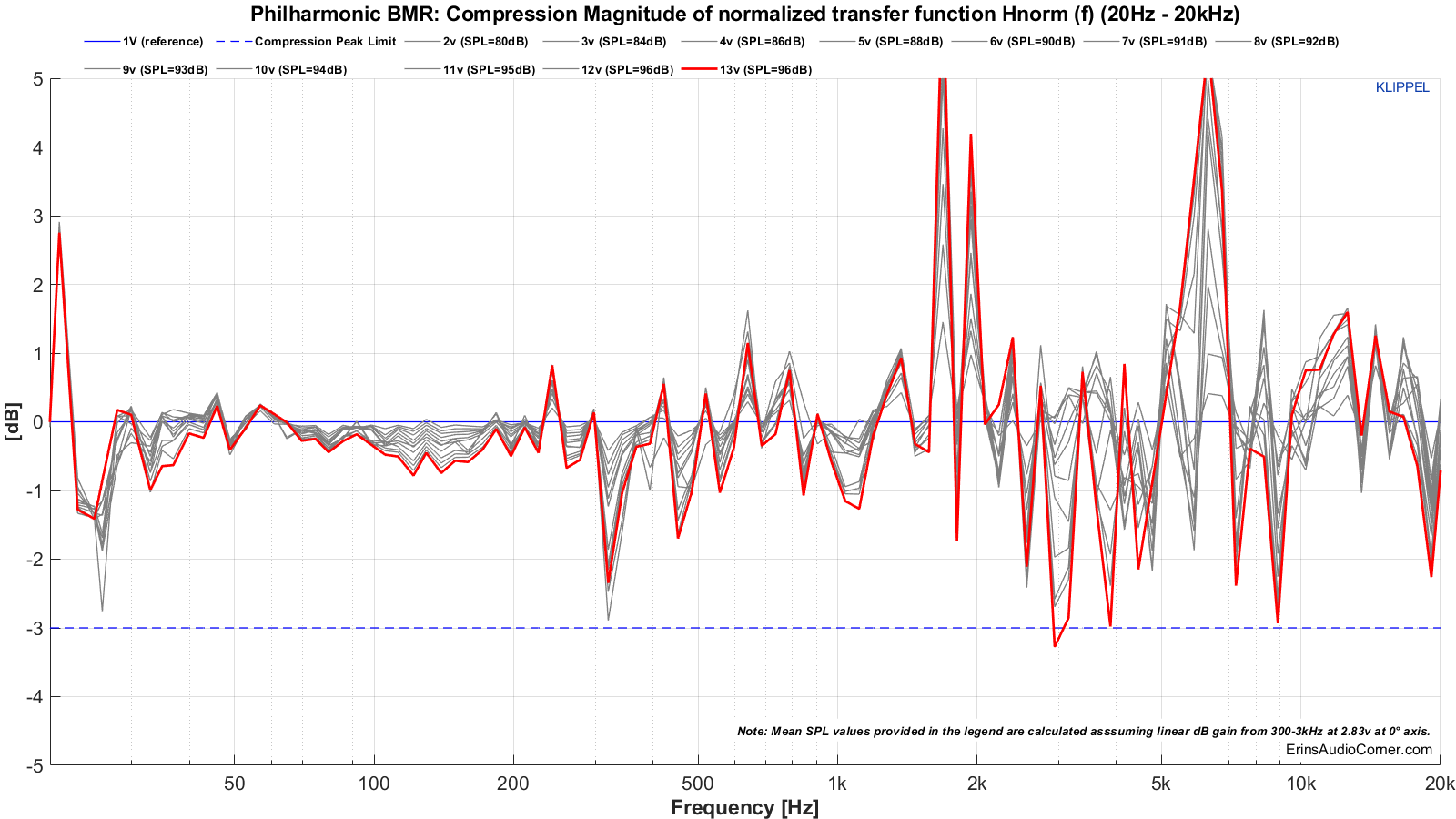
Test 1: 20Hz to 20kHz

Multitone compression testing. The red line shows the final measurement where either distortion and/or compression failed. The voltage just before this is used to help determine the maximum SPL.

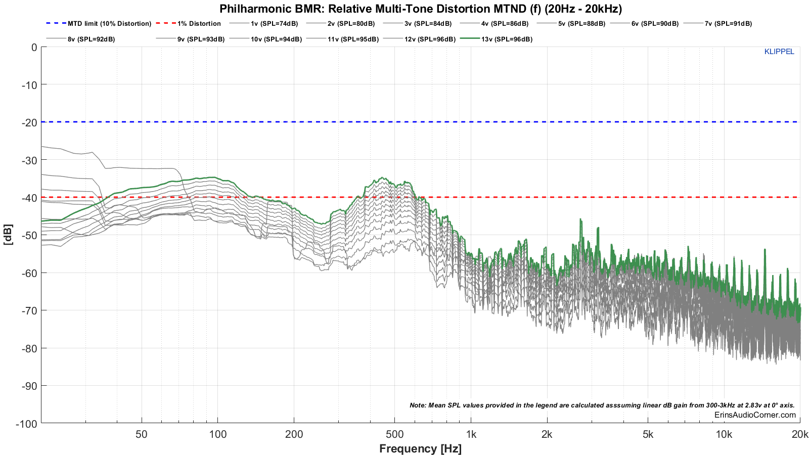
Multitone distortion testing. The dashed blue line represents the -20dB (10% distortion) threshold for failure. The dashed red line is for reference and shows the 1% distortion mark (but has no bearing on pass/fail). The green line shows the final measurement where either distortion and/or compression failed. The voltage just before this is used to help determine the maximum SPL.

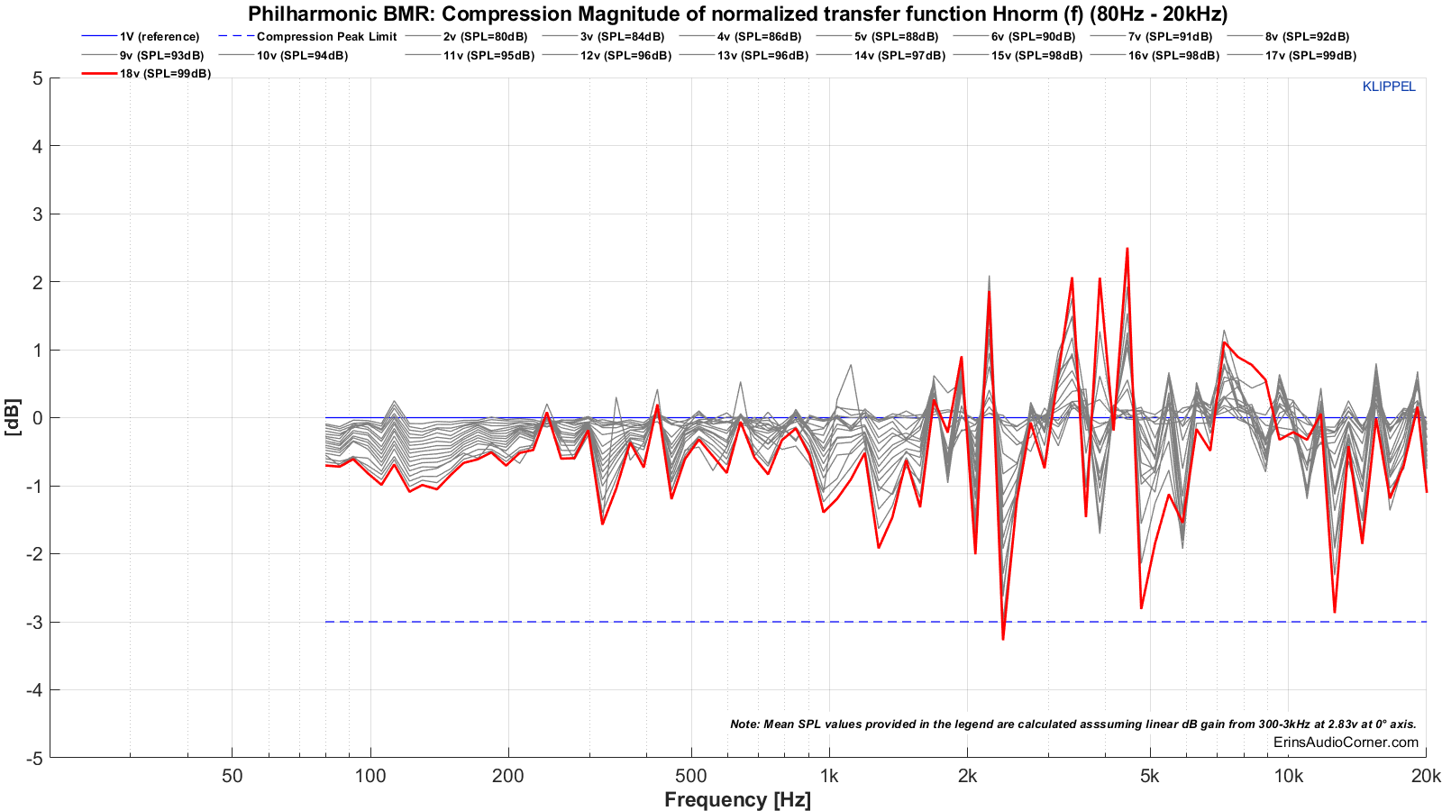
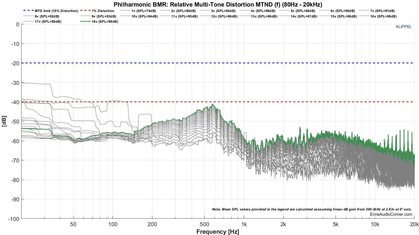
Test 2: 80Hz to 20kHz

Multitone compression testing. The red line shows the final measurement where either distortion and/or compression failed. The voltage just before this is used to help determine the maximum SPL.

The above data can be summed up by looking at the tables above but is provided here again:

Max SPL for 20Hz to 20kHz is approximately 96dB @ 1 meter. The compression threshold was exceeded above this SPL.
Max SPL for 80Hz to 20kHz is approximately 99dB @ 1 meter. The compression threshold was exceeded above this SPL.

Extra Measurements:

Nearfield measurements.

Mic placed about 0.50 inches - relative to the baffle - from each drive unit and port. While I tried to make these as accurate in SPL as I could, I cannot guarantee the relative levels are absolutely correct so I caution you to use this data as a guide but not representative of actual levels (measuring in the nearfield makes this hard as a couple millimeters’ difference between measurements can alter the SPL level).

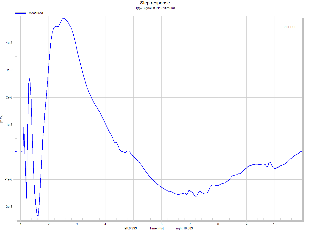
Step-Response.

Not Zoomed:

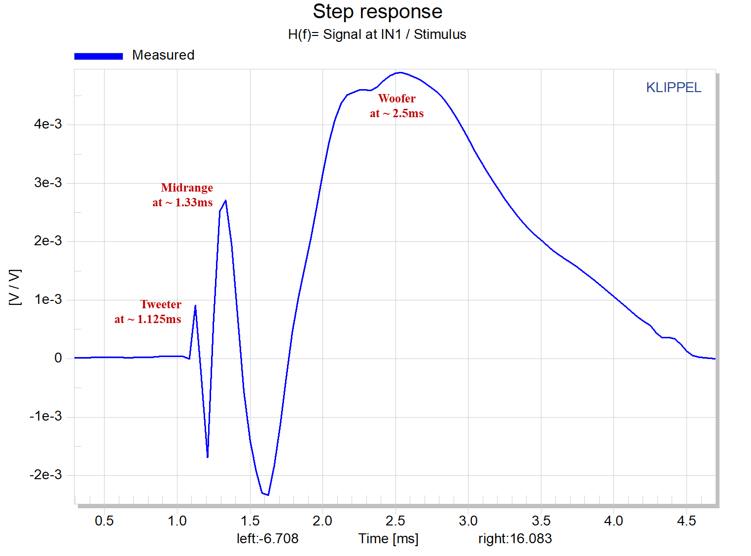
Zoomed and annotated for the arrival time of each drive-unit’s impulse. You can see the drivers are not time-aligned and arrive distinctly separately. The difference in time between the woofer (2.5ms) and the midrange (1.33ms) is approximately 1.2ms. To put this in perspective, 1.2ms is approximately 16 inches.

Subjective Evaluation:

Before I dive in to the subjective feedback let me first give you the layout of my room…

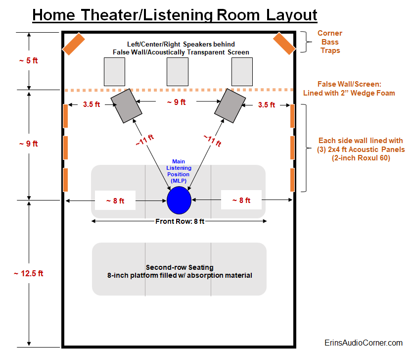
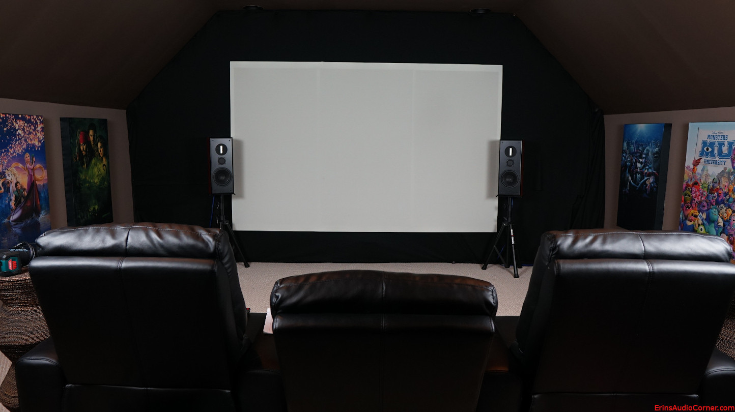
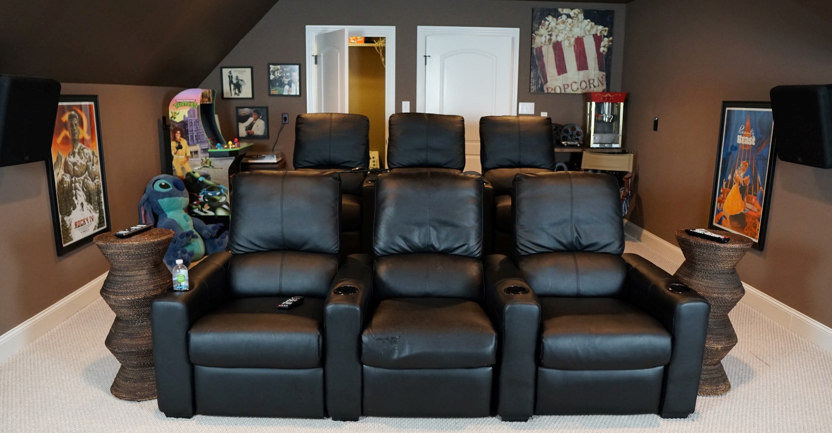
If the false wall part is odd to you, here's some background. I don't like seeing speakers when watching a movie. So, I built a false wall and used an acoustically transparent screen with speakers behind it. The wall is only 2x4's; no panels of wood or anything. Just a skeleton of a wall to give me something to attach the screen and acoustic treatment to. There is 2-inch wedge foam affixed to the 2x4 studs and between the false wall and back of the room are the front speakers (L/C/R & 18-inch subwoofers).

My demo music:

Title	Artist	Album
Enjoy The Silence	Depeche Mode	Best Of Depeche Mode, Vol. 1
Higher Love	Steve Winwood	Back In The High Life (MFSL UDCD-611)
24K Magic	Bruno Mars	24K Magic
Magic	The Cars	Heartbeat City (MFSL)
Everlasting Love	Howard Jones	The Best of Howard Jones
Kodachrome	Paul Simon	There Goes Rhymin’ Simon
Everybody Wants To Rule The World	Tears for Fears	Songs from the Big Chair (2014 Deluxe Edition - Disc 1)
Know Your Enemy	Rage Against The Machine	Rage Against The Machine (Hybrid SACD)
Doo Wop (That Thing)	Lauryn Hill	The Miseducation of Lauryn Hill
Tell Yer Mama	Norah Jones	The Fall
Don’t Save Me	HAIM	Days Are Gone
He Mele No Lilo	Mark Keali’i Ho’omalu and Kamehameha Schools Children’s Chorus	Lilo And Stitch
Wrapped Around Your Finger	The Police	Synchronicity
Sledgehammer	Peter Gabriel	So
Feel It Still	Portugal. The Man	Woodstock
Free Fallin	John Mayer	Where The Light Is
Whiplash	The Swampers	Muscle Shoals Has Got The Swampers

Note: I don’t generally audition speakers with the typical “audiophile” music. I have thousands of high-quality albums ranging from pop to metal to jazz and all around. I don’t typically listen to “audiophile” music because I just don’t enjoy it. It is far more important that your evaluation music be something you are familiar with than it is to be esoteric for the sake of being esoteric. You also want to listen to music you enjoy because auditioning a stereo system shouldn’t feel like a chore. Such is the case in my evaluations. Besides, the subjective evaluation is purely to help tie to the objective data and make sense of what I am hearing to help you all get an understanding of how relevant the data is. As you will see below, my music selection did a great job at providing enough range for me to identify the issues that readily appear in the data.

Subjective Analysis Setup:

The speaker was aimed on-axis with the vertical listening axis on the tweeter axis.
I used Room EQ Wizard (REW) and my calibrated MiniDSP UMIK-1 to get the volume on my AVR relative to what the actual measured SPL was in the MLP (~11 feet from the speakers). I varied it between 85-90dB, occasionally going up to the mid 90’s to see what the output capability was. In a poll I found most listen to music in this range.
All speakers are provided a relatively high level of Pseudo Pink-Noise for a day or two - with breaks in between - in order to calm any “break-in” concerns.
I demoed these speakers without a crossover and without EQ.
Components: Oppo BDP-103 playing music off my thumb drive feeding signal via HDMI to a Denon AVR-X4000 which then feeds in to a refurbished Adcom GFA-545 for power.

I listened to these speakers and made my subjective notes before I started measuring objectively. I did not want my knowledge of the measurements to influence my subjective opinion. This is important because I want to try to correlate the objective data with what I hear in my listening space in order to determine the validity of the measurement process. I try to do a few listening sessions over a couple days so I can give my ears a break and come back “fresh”.

In the interest of time and due to no feedback discussing these matters, I am not providing photos of my notes (seems like no one cares and no sense in wasting my time if it’s not important to anyone). I did complete in-room measurements but sold the laptop without saving the results to my external drive so I am unable to provide those at this moment.

Here’s the rundown of my subjective notes (in quotes) and where it fits with objective:

Overall, I found the max SPL I could drive the speakers to was around 98-100dB at my listening position, depending on the music. Which is quite loud at 11.5 feet! The tell-tale for me here was the woofer ran out of mechanical excursion listening to Lauryn Hill’s “Doo Wop”. I didn’t notice any annoying distortion with the tracks I used. I did hear some things that sounded different and now having seen the data, I wonder if the increased harmonic distortion between 2-4kHz might have been a contributor but I cannot say with any degree of certainty that it was.
Depeche Mode’s “Enjoy The Silence”: really nice punch in the bass. When the lead singer says “… oh my little girl…” I heard modulation in his voice that I have never heard before. That’s a good thing. It means, at least to me, the resolution of the speaker is extremely high. This was a common trend throughout the rest of my demo.
Steve Winwood’s “Higher Love”: The panning drums on this track were very nice. I wrote “WOW” in my notes. I was jamming to this track at about 95dB and it sounded incredible. Chaka Khan’s voice at the end literally gave me goosebumps. Goosebumps. I did note there was something in the 800Hz region that I hadn’t noticed before and I didn’t have a specific way to describe it. It stood out; I wasn’t sure if it was good or bad. Looking at the data, I believe I may have been hearing the resonance I discussed earlier.
The Cars “Magic”: Missing some “crackle (10k - 12kHz?)". Looking at the data shows a falloff in response above 10kHz.
The Police “Wrapped Around Your Finger”: This speaker reproduced the bass line better than anything I’ve ever heard to date. I noted that it seemed a bit excessive in the 2-3kHz region, though. I see in the data that the off-axis response is a bit brighter in this region but I’m not sure if that’s the reason I heard what I heard or not.
Peter Gabriel’s “Sledgehammer”: I could hear inflection in his voice that I’d never heard before which I felt was, again, attributed to the HF response.
Portugal The Man’s “Feel It Still”: The chord progression on this track… I could feel it coming at me. Like it was coming out of the speakers. Crazy.
John Mayer’s cover of Tom Petty’s “Free Fallin”: I see audiophile types say “you want to feel like you’re in the audience”. My response is typically “yea, if the recording is made in a way that will allow it”. The easy example is a singer with auto-tune: he/she shouldn’t sound “real” at all. But, sure, if the recording is of good quality and “real” was the objective then using that as a reference for a real sound is just fine. I feel this recording is one of those. But I haven’t heard a speaker yet that “puts me there” like these do. It was so cool, I even got my wife to listen in the sweet spot. Of course, she said “sounds cool” and went on her way. But the next day she had that song on one of her playlists. So… I take that as a win for this speaker.
Paul Simon “Kodachrome”: Drums on the left side of the stage were clearly behind the speaker. Though, I did find something to be a bit resonant in the 250-300Hz region. The majority of the data doesn’t reveal any reason for me having heard this. However, when I look back at the normalized horizontal response I can see a small bump right in this region as the response trends off-axis. I am honestly very impressed that a) I heard this and b) there is correlating data. I keep saying… if the data doesn’t show it then either something is wrong or you’re not looking at the right data. This is a prime example of the latter.
Tears For Fears “Everybody Wants To Rule The World”: perfect ~160hz vocal tone. “Behind You”… “Be-hind”… the “beee” portion of this word sounded a bit boomy. Might be the 250-300Hz resonance noted above. Might also be my imagination. Or might be the way it is supposed to sound. I believe it’s resonance, though. The breakdown portion starting around 2:40 has a three-chord progression; low notes. I have listened to this song thousands of times… thousands… it is my favorite song of all time… and I have never noticed the “pluck” of those notes until I heard it on these speakers. Of course, now that I’ve heard it, I notice it on other speakers… but I credit the BMRs for making that possible.
Norah Jones “Tell Yer Mama”: Backup vocalist on the left is as wide as my room with the speakers placed about 3.5 feet from the side walls.

I chose not to run Dirac Live with these speakers due to time constraints. But with a little bit of EQ on the 4-8kHz region (where I felt it was about 1dB too high) and with room correction, I can only imagine how much better my listening impression would have been.

Bottom Line

These speakers are awesome. The tonality revealed things in songs I’d never heard before (in only one case did I find that to be a negative). The resolution reveals little details such as slight inflections in voices and even accentuates the breathing-in of a vocalist before they begin their next line. It was a new experience for me to hear these kind of details. The soundstage is incredibly large and well balanced and the reflections in the room help to extend the soundstage to a size I’ve yet to hear from another speaker to date.

For the kit price of about $1000, I can’t imagine anything coming close to the value of this speaker in DIY form. I would have no qualms at all paying the kit price and ordering the flat pack and assembling this myself for about $1500/pair. And if I had more money and less time I wouldn’t mind ordering them complete from Salk. No matter what your experience level or desire to build, I think these speakers are a no brainer for their price.

However, I would like to hear what these speakers can do if one was to cover the tweeter so as to make it a small square rather than as tall as it is. That would theoretically bring the beaming point up to match the horizontal dispersion pattern and I would really be interested to see how that additional vertical window of dispersion would help (or potentially hurt) these speakers.

Objectively speaking, one potentially large concern (emphasis on potentially; your mileage may vary based on use) is the very low sensitivity of 83.2dB at 2.83v/1m. Therefore, I also would like to see what this speaker would be like if the BMR had a higher sensitivity. When I tested one of Tectonics’ 2 inch BMR speakers some years back (link here) I was very impressed with the linearity of response even beyond the typical beaming point. However, the abysmal sensitivity of that speaker kept it from being one I could recommend for typical DIY use. The BMR used in this speaker, too, has a very low sensitivity and therefore all the other drive units’ output capability are brought down in level to match it. The Scan woofer used here has a sensitivity higher sensitivity of about 87dB but baffle step compensation would also bring the sensitivity down some. Therefore, the woofer would need to be upgraded to something with higher sensitivity. The Scan-Speak Illuminator would be a pretty good alternative, considering it has a bit more linear excursion than the one used in this speaker design. Of course, the Illuminator is an easy $100/driver more than the Classic woofer. Basically, if the sensitivity of this speaker were higher… that would make for a very top-shelf speaker but would also drive the cost up a bit more and you begin to reach the point where the value (price per performance) may take a hit.

Another aspect that would be interesting to investigate is the time-alignment of the drivers. As shown previously, these drivers are not time-aligned. Personally speaking, it’s not easy for me to notice smaller differences in time alignment in absolute terms. But, when I have a DSP and the ability to adjust time delay manually using pink noise or test tones (for high frequency and low frequency, respectively) I almost always can manually nail the correct time delay values when I compare to a microphone measurement. So, while maybe not incredibly obvious, timing does matter and I - as well as others I know - can hear when a drive unit is in time/phase with another one when given the opportunity to make adjustments manually. Correct time alignment at the crossover always helps the coherency; that’s how I am able to detect when I am “in time” or not via DSP settings. So, I have to believe that if this speaker had all the drivers aligned in time that the result would be another level of improvement.

At any rate, kudos to Mr. Murphy on a very well designed speaker!

Support the Cause

If you like what you see here and want to help support the cause you might be interested in joining my Patreon, here. You can also contribute via PayPal (the big yellow button below).

Your support helps me pay for new items to test, hardware, miscellaneous items and costs of the site’s server space and bandwidth. All of which I otherwise pay out of pocket. So, if you can help chip in a few bucks, know that it is very much appreciated.

You can also join my Facebook and YouTube pages via the links at the bottom of the page if you’d like to follow along with updates.

Thanks!