Foreword / YouTube Video Review
These speakers were loaned to me by their owner who had them dropped shipped to me from a retailer.
The review on this website is a brief overview and summary of the objective performance of this speaker. It is not intended to be a deep dive. Moreso, this is information for those who prefer “just the facts” and prefer to have the data without the filler. The video below has more discussion.
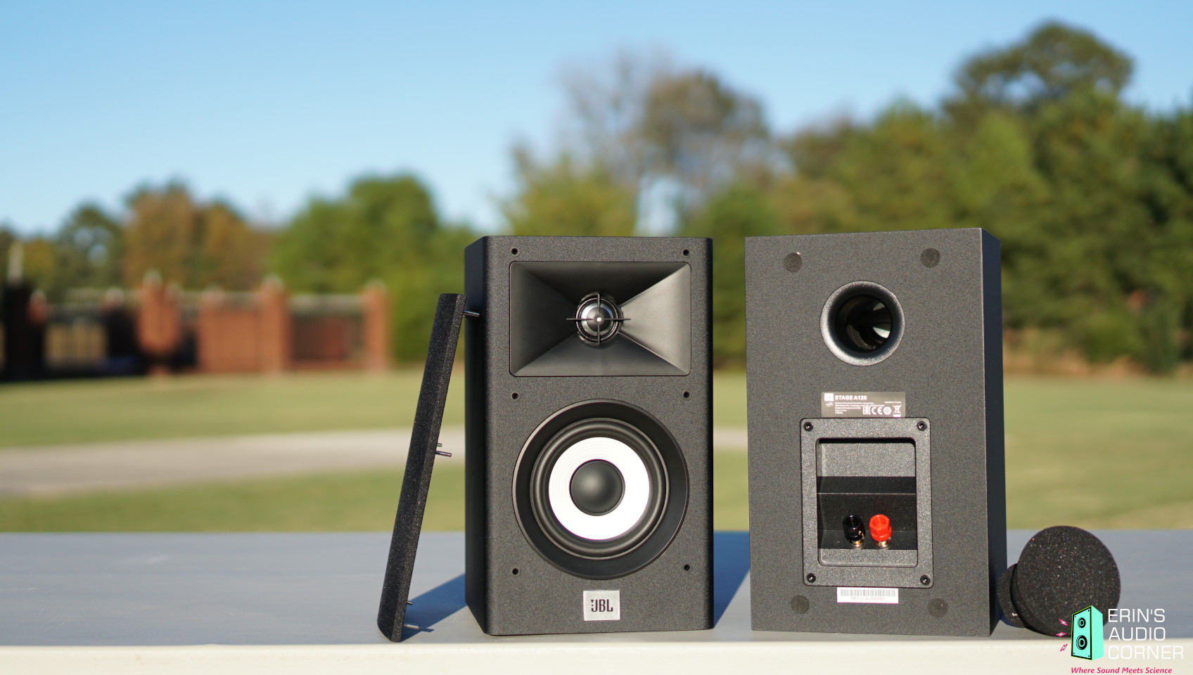
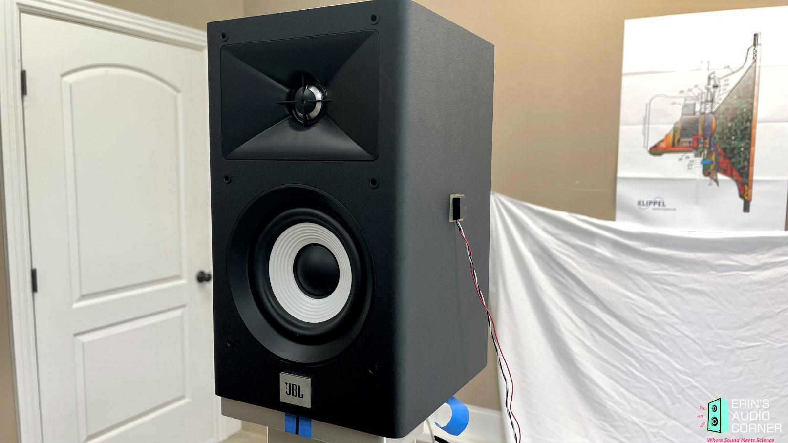
Information and Photos
Some specs from a retailer (note: the manufacturer’s blurb was about the lineup; not this specific speaker):
Need a budget-friendly set of surround speakers for your home theater? Or a compact stereo pair to bring music to a tight spot? Consider the JBL A120. It’s the smallest speaker in JBL’s new Stage lineup, but it benefits from the company’s long and rich history of making speakers. JBL paid particular attention to the design of the enclosure on these speakers, aiming to craft a non-resonant cabinet with rigid walls and internal bracing so that you hear your music and movies as they were meant to be heard. Expertly built drivers The 1" aluminum dome tweeter is mounted in an HDI (High Definition Imaging) waveguide that was designed for the JBL Professional M2 Master Reference Monitor. This flared shape helps smooth the transition from woofer to tweeter for a broad sweet spot and clear high-frequency detail. Each speaker’s striking white 4-1/2" woofer is made of a stiff-but-lightweight polycellulose material to deliver solid bass for its size. A rear-panel port reinforces bass performance.
Price is approximately $200 USD for the pair.
If you are interested in purchasing this speaker (though, it’s not a speaker I would necessarily recommend), please consider using the following affiliate link which earns me a small commission at no additional cost to you: Buy from Amazon
CTA-2034 (SPINORAMA) and Accompanying Data
All data collected using Klippel’s Near-Field Scanner. The Near-Field-Scanner 3D (NFS) offers a fully automated acoustic measurement of direct sound radiated from the source under test. The radiated sound is determined in any desired distance and angle in the 3D space outside the scanning surface. Directivity, sound power, SPL response and many more key figures are obtained for any kind of loudspeaker and audio system in near field applications (e.g. studio monitors, mobile devices) as well as far field applications (e.g. professional audio systems). Utilizing a minimum of measurement points, a comprehensive data set is generated containing the loudspeaker’s high resolution, free field sound radiation in the near and far field. For a detailed explanation of how the NFS works and the science behind it, please watch the below discussion with designer Christian Bellmann:
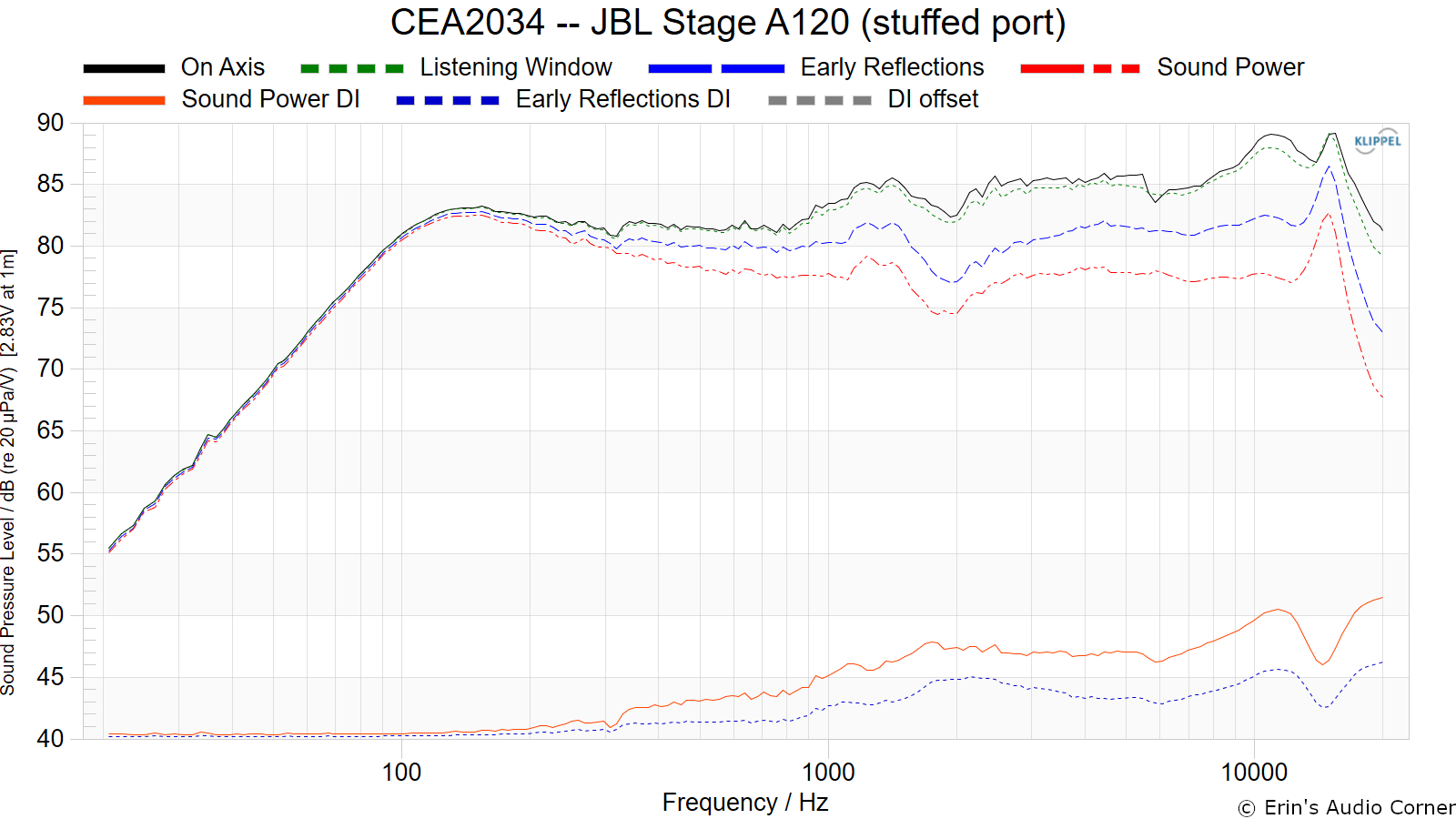
The reference plane in this test is at the tweeter. Testing was performed without the grille in place. Initial testing was performed with the port open (not stuffed). However, another round of testing was performed with the port stuffed and the results will be clearly identified in the results below near the bottom.
Measurements are provided in a format in accordance with the Standard Method of Measurement for In-Home Loudspeakers (ANSI/CTA-2034-A R-2020). For more information, please see this link.
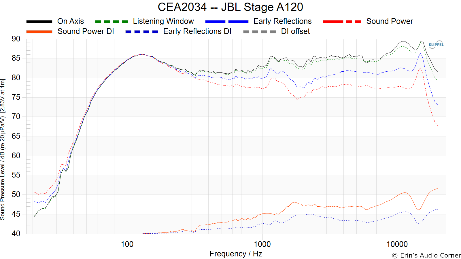
CTA-2034 / SPINORAMA:
The On-axis Frequency Response (0°) is the universal starting point and in many situations it is a fair representation of the first sound to arrive at a listener’s ears.
The Listening Window is a spatial average of the nine amplitude responses in the ±10º vertical and ±30º horizontal angular range. This encompasses those listeners who sit within a typical home theater audience, as well as those who disregard the normal rules when listening alone.
The Early Reflections curve is an estimate of all single-bounce, first-reflections, in a typical listening room.
Sound Power represents all of the sounds arriving at the listening position after any number of reflections from any direction. It is the weighted rms average of all 70 measurements, with individual measurements weighted according to the portion of the spherical surface that they represent.
Sound Power Directivity Index (SPDI): In this standard the SPDI is defined as the difference between the listening window curve and the sound power curve.
Early Reflections Directivity Index (EPDI): is defined as the difference between the listening window curve and the early reflections curve. In small rooms, early reflections figure prominently in what is measured and heard in the room so this curve may provide insights into potential sound quality.
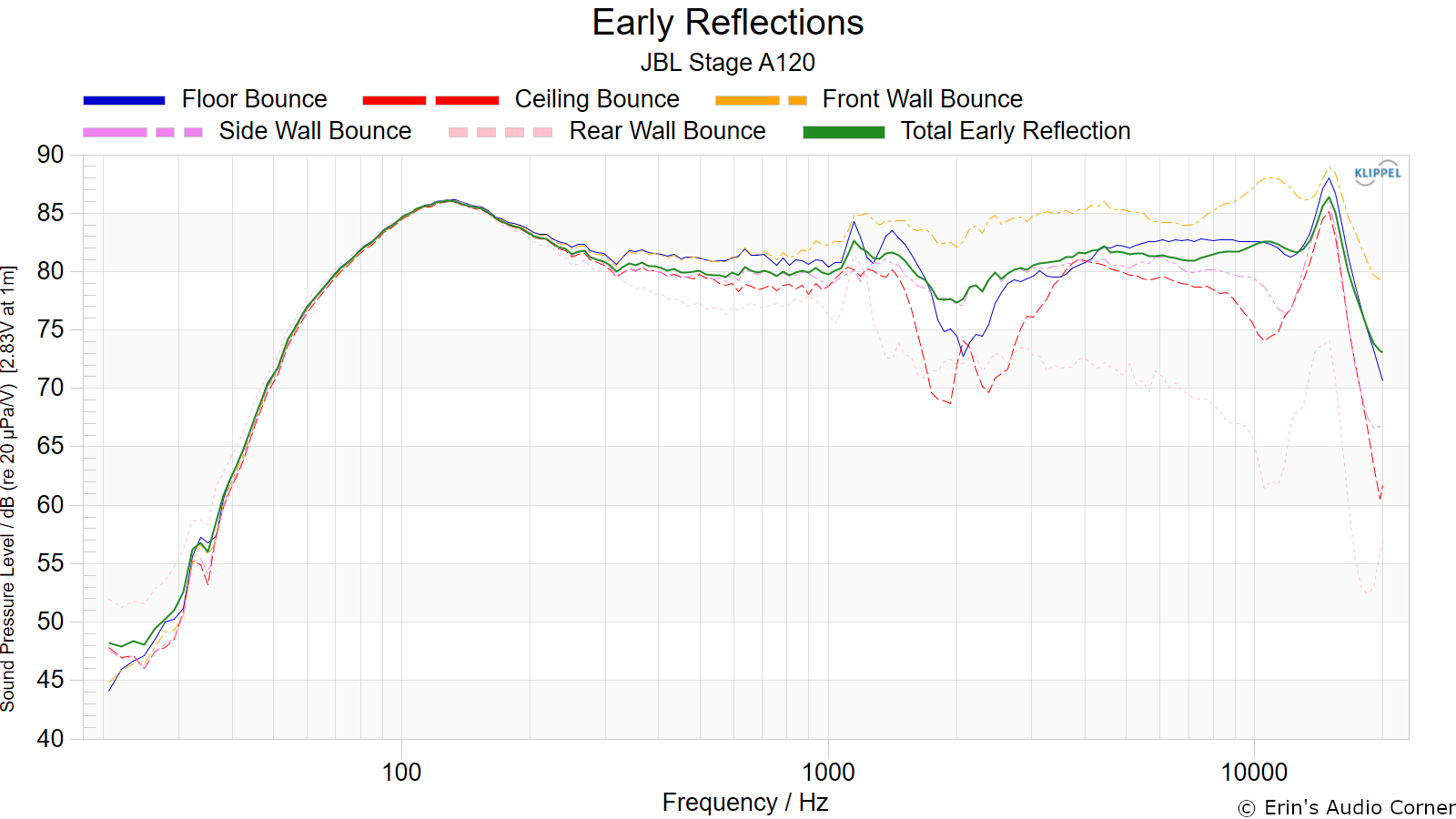
Early Reflections Breakout:
Floor bounce: average of 20º, 30º, 40º down
Ceiling bounce: average of 40º, 50º, 60º up
Front wall bounce: average of 0º, ± 10º, ± 20º, ± 30º horizontal
Side wall bounces: average of ± 40º, ± 50º, ± 60º, ± 70º, ± 80º horizontal
Rear wall bounces: average of 180º, ± 90º horizontal
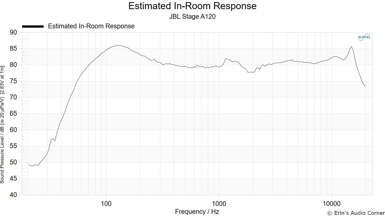
Estimated In-Room Response:
In theory, with complete 360-degree anechoic data on a loudspeaker and sufficient acoustical and geometrical data on the listening room and its layout it would be possible to estimate with good precision what would be measured by an omnidirectional microphone located in the listening area of that room. By making some simplifying assumptions about the listening space, the data set described above permits a usefully accurate preview of how a given loudspeaker might perform in a typical domestic listening room. Obviously, there are no guarantees, because individual rooms can be acoustically aberrant. Sometimes rooms are excessively reflective (“live”) as happens in certain hot, humid climates, with certain styles of interior décor and in under-furnished rooms. Sometimes rooms are excessively “dead” as in other styles of décor and in some custom home theaters where acoustical treatment has been used excessively. This form of post processing is offered only as an estimate of what might happen in a domestic living space with carpet on the floor and a “normal” amount of seating, drapes and cabinetry.
For these limited circumstances it has been found that a usefully accurate Predicted In-Room (PIR) amplitude response, also known as a “room curve” is obtained by a weighted average consisting of 12 % listening window, 44 % early reflections and 44 % sound power. At very high frequencies errors can creep in because of excessive absorption, microphone directivity, and room geometry. These discrepancies are not considered to be of great importance.
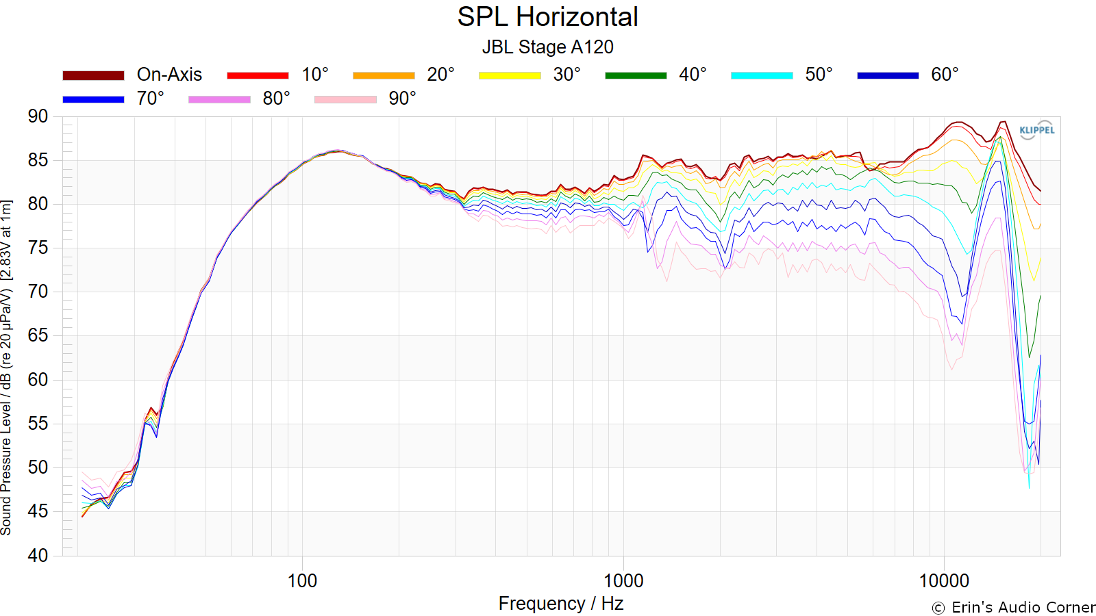
Horizontal Frequency Response (0° to ±90°):
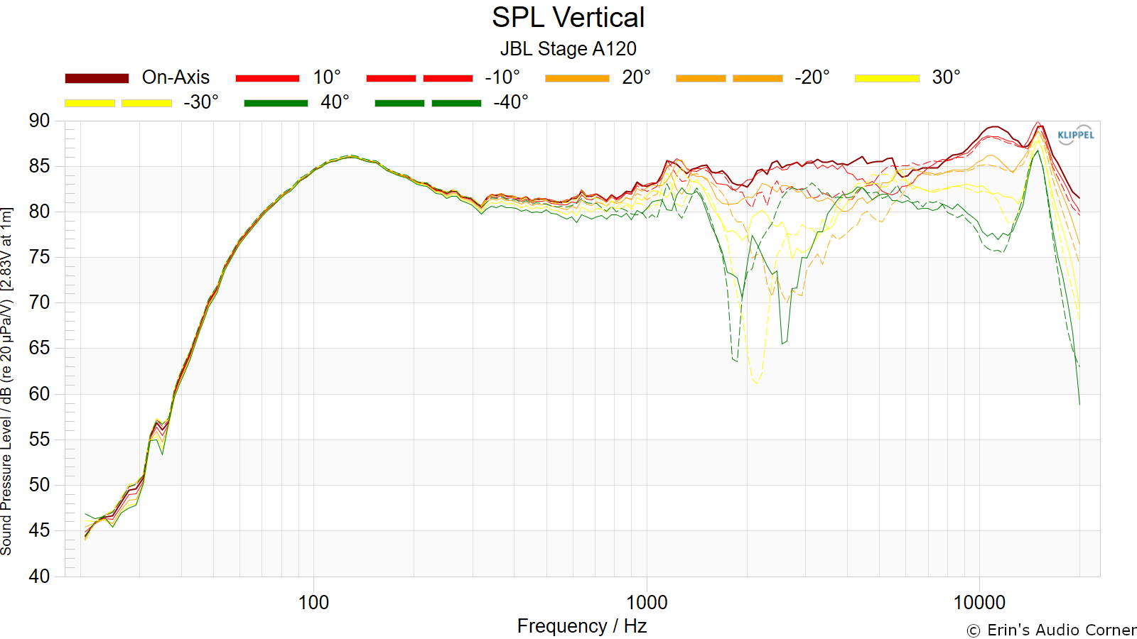
Vertical Frequency Response (0° to ±40°):
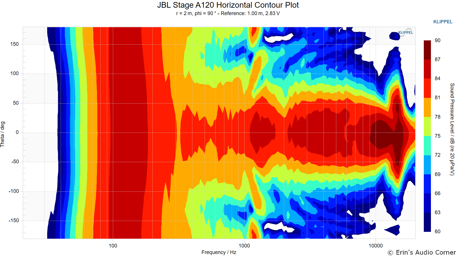
Horizontal Contour Plot (not normalized):
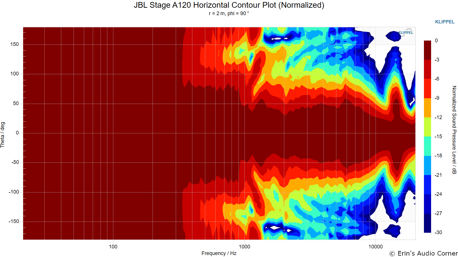
Horizontal Contour Plot (normalized):
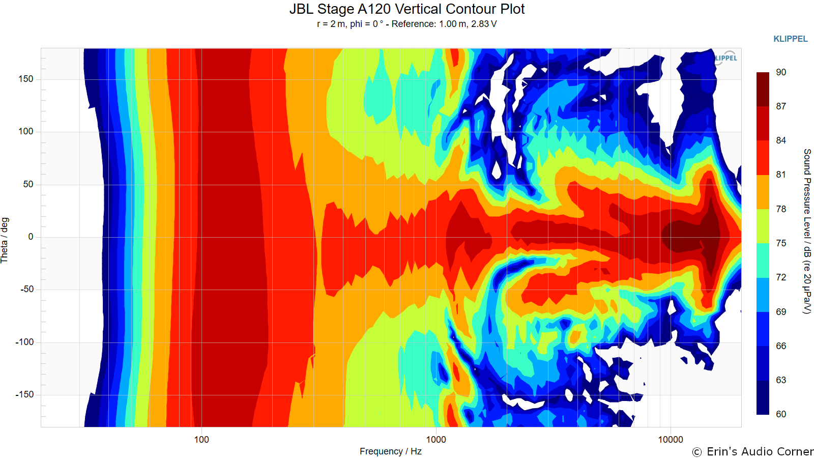
Vertical Contour Plot (not normalized):
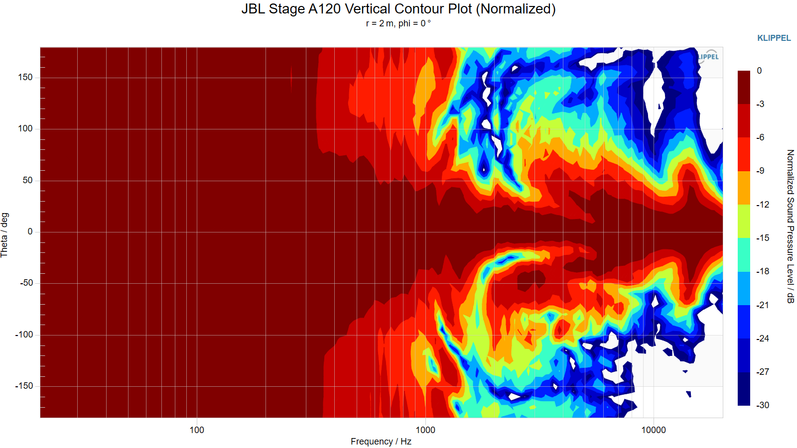
Vertical Contour Plot (normalized):
“Globe” Plots
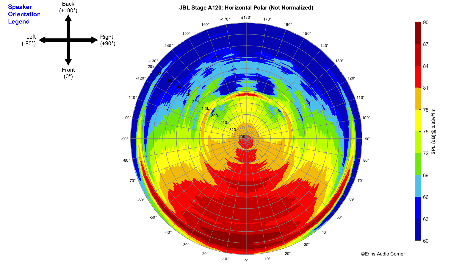
Horizontal Polar (Globe) Plot:
This represents the sound field at 2 meters - above 200Hz - per the legend in the upper left.
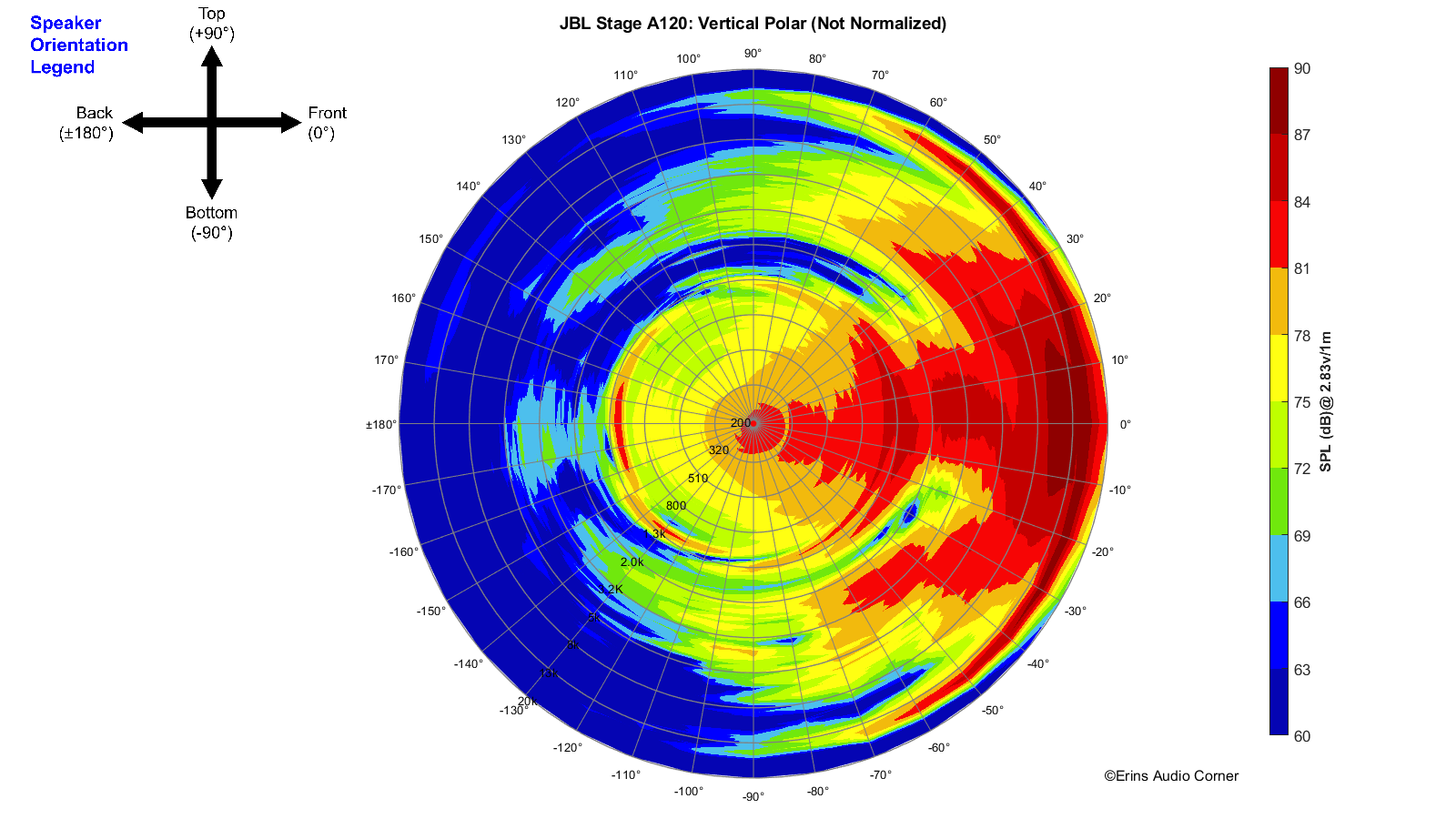
Vertical Polar (Globe) Plot:
This represents the sound field at 2 meters - above 200Hz - per the legend in the upper left.
Additional Measurements
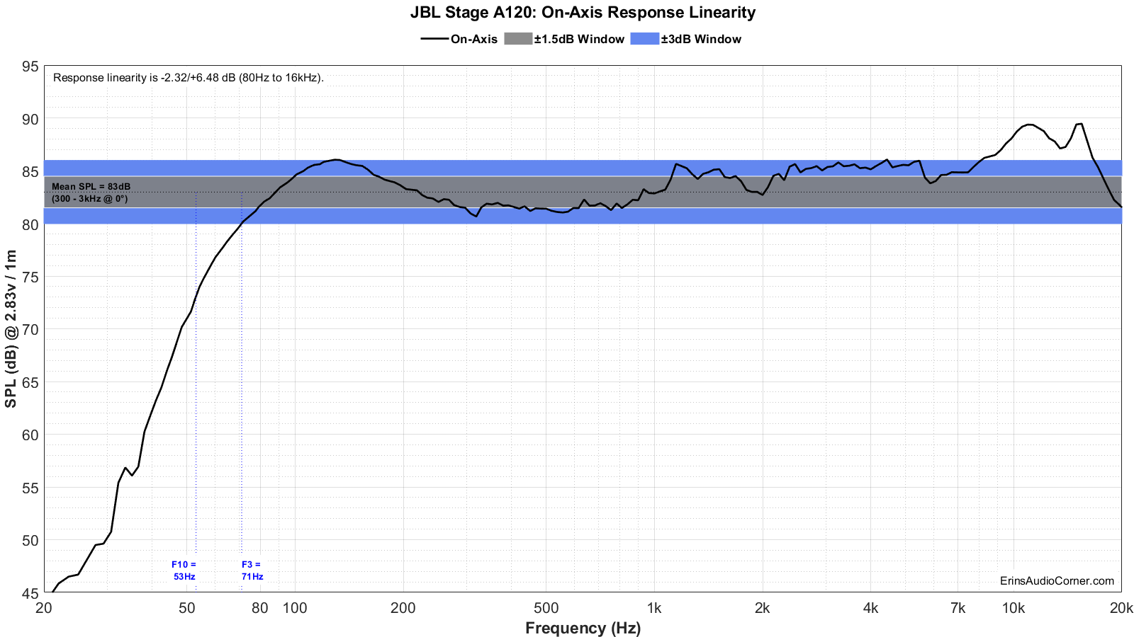
On-Axis Response Linearity
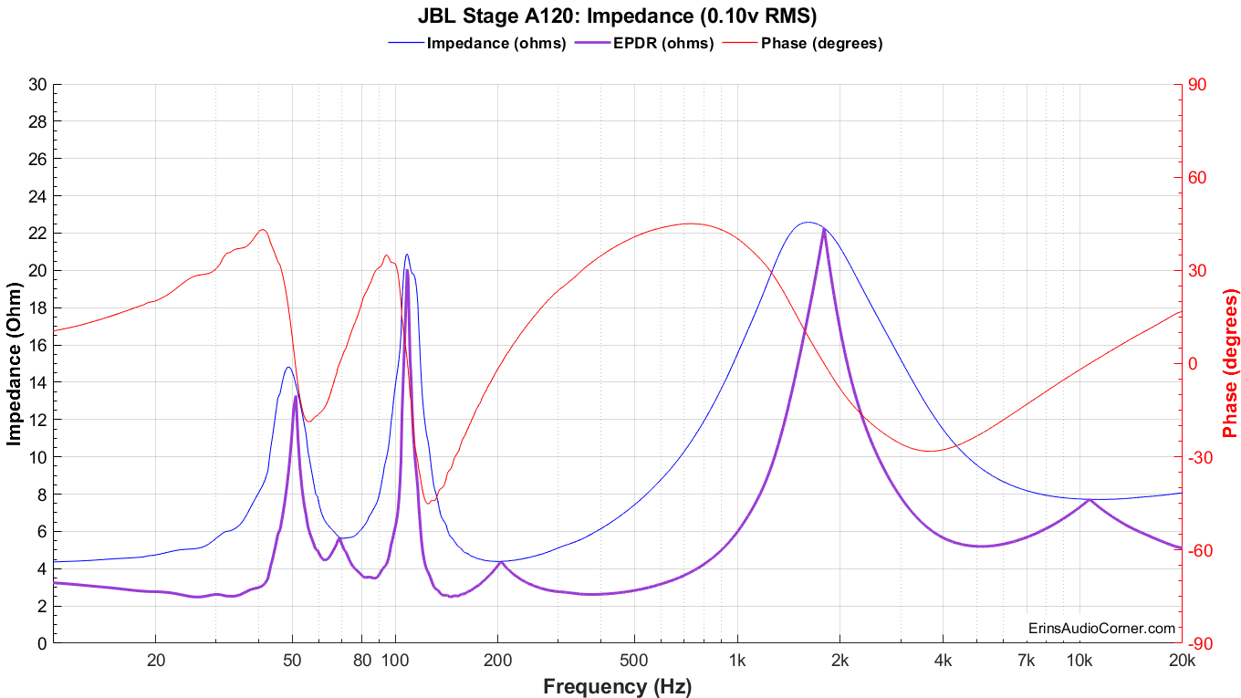
Impedance Magnitude and Phase + Equivalent Peak Dissipation Resistance (EPDR)
For those who do not know what EPDR is (ahem, myself until 2020), Keith Howard came up with this metric which he defined in a 2007 article for Stereophile as:
… simply the resistive load that would give rise to the same peak device dissipation as the speaker itself.
A note from Dr. Jack Oclee-Brown of Kef (who supplied the formula for calculating EPDR):
Just a note of caution that the EPDR derivation is based on a class-B output stage so it’s valid for typical class-AB amps but certainly not for class-A and probably has only marginal relevance for class-D amps (would love to hear from a class-D expert on this topic).
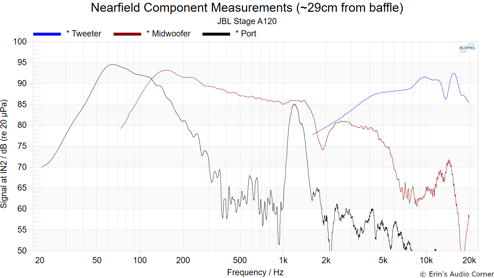
Near-Field Response
Nearfield response of individual drive units:
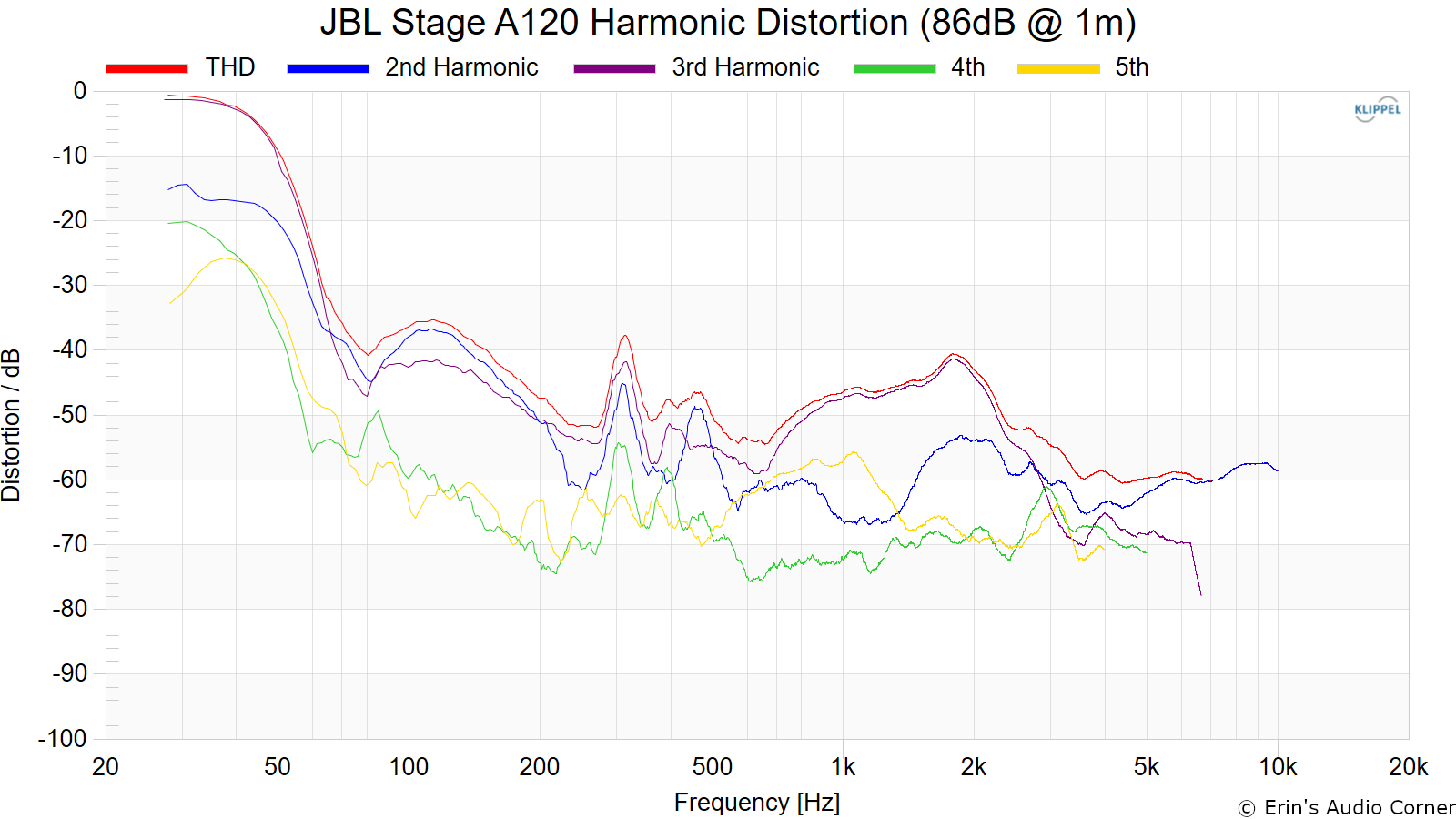
Harmonic Distortion
Harmonic Distortion at 86dB @ 1m:
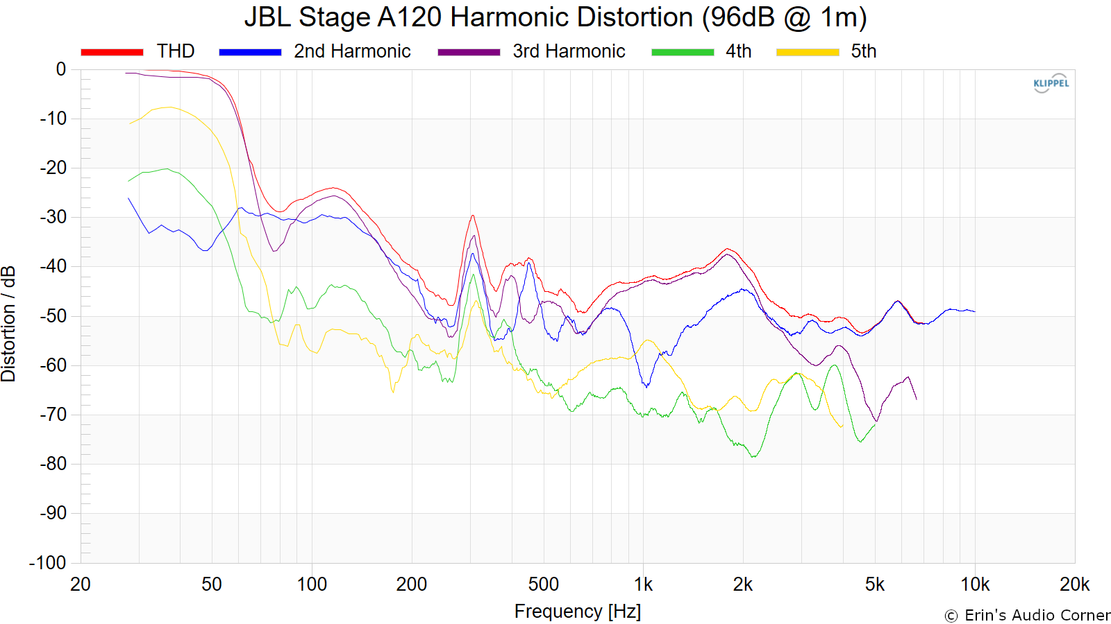
Harmonic Distortion at 96dB @ 1m:
Dynamic Range (Instantaneous Compression Test)
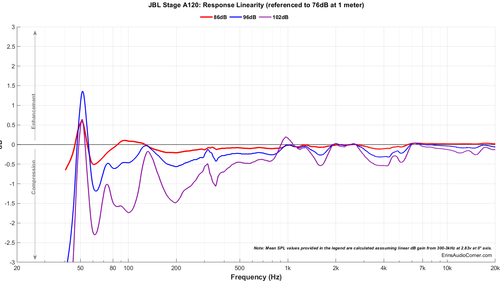
The below graphic indicates just how much SPL is lost (compression) or gained (enhancement; usually due to distortion) when the speaker is played at higher output volumes instantly via a 2.7 second logarithmic sine sweep referenced to 76dB at 1 meter. The signals are played consecutively without any additional stimulus applied. Then normalized against the 76dB result.
The tests are conducted in this fashion:
- 76dB at 1 meter (baseline; black)
- 86dB at 1 meter (red)
- 96dB at 1 meter (blue)
- 102dB at 1 meter (purple)
The purpose of this test is to illustrate how much (if at all) the output changes as a speaker’s components temperature increases (i.e., voice coils, crossover components) instantaneously.
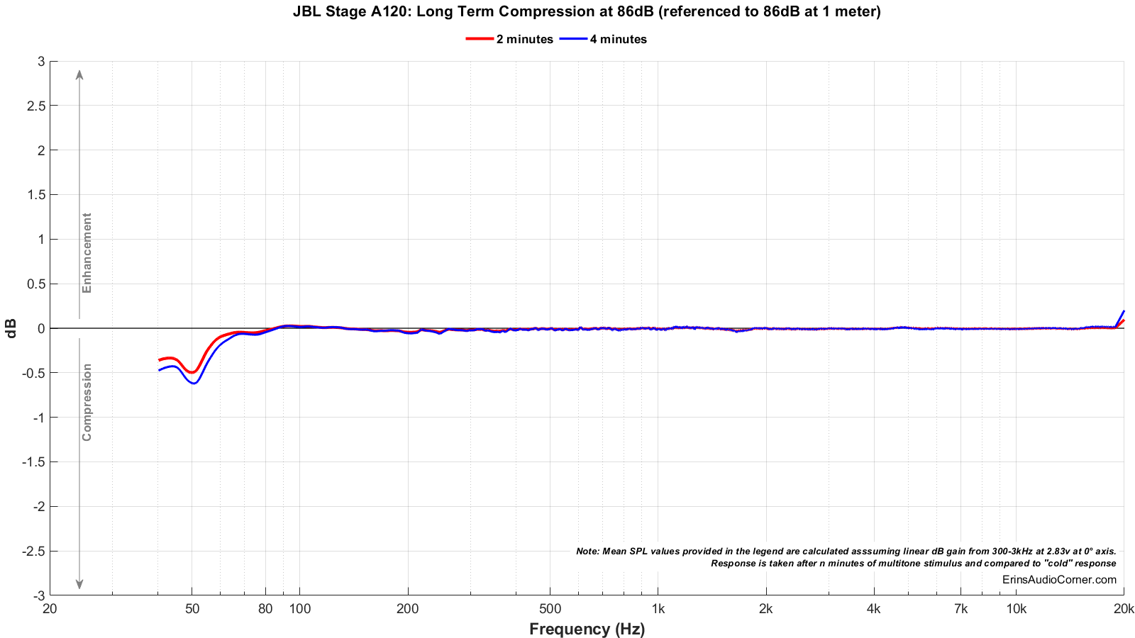
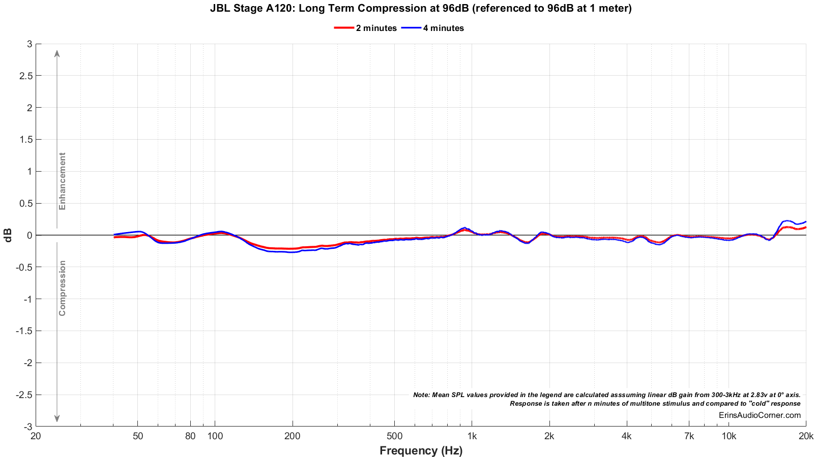
Long Term Compression Tests
The below graphics indicate how much SPL is lost or gained in the long-term as a speaker plays at the same output level for 2 minutes, in intervals. Each graphic represents a different SPL: 86dB and 96dB both at 1 meter.
The purpose of this test is to illustrate how much (if at all) the output changes as a speaker’s components temperature increases (i.e., voice coils, crossover components).
The tests are conducted in this fashion:
- “Cold” logarithmic sine sweep (no stimulus applied beforehand)
- Multitone stimulus played at desired SPL/distance for 2 minutes; intended to represent music signal
- Interim logarithmic sine sweep (no stimulus applied beforehand) (Red in graphic)
- Multitone stimulus played at desired SPL/distance for 2 minutes; intended to represent music signal
- Final logarithmic sine sweep (no stimulus applied beforehand) (Blue in graphic)
The red and blue lines represent changes in the output compared to the initial “cold” test.
CTA-2034 (SPINORAMA) in Sealed Configuration (Port Stuffed with provided foam)
Enclosure Resonance Insight
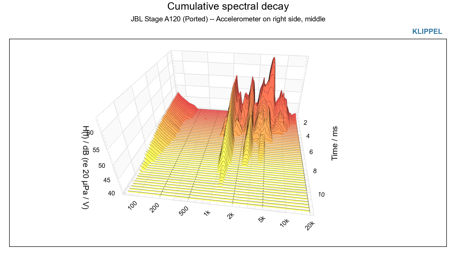
(Cabinet Vibration - Cumulative Spectral Decay (CSD))
Noting there were signs of resonance in the 1-2kHz region, I proceeded to test what the source was. Given the strong peak measured at the nearfield of the port, I first checked to see if the port was the culprit. I stuffed the port and found no meaningful difference made (compare the above “Port Stuffed” SPIN results with that of the original SPIN results). Therefore, I wouldn’t say the port itself is at fault.
I then compared the CSD of both aforementioned results (provided below). First ported, then sealed. Interestingly, the 1kHz resonance is subdued by about 3ms but the other series of resonances appear unaffected. See below.
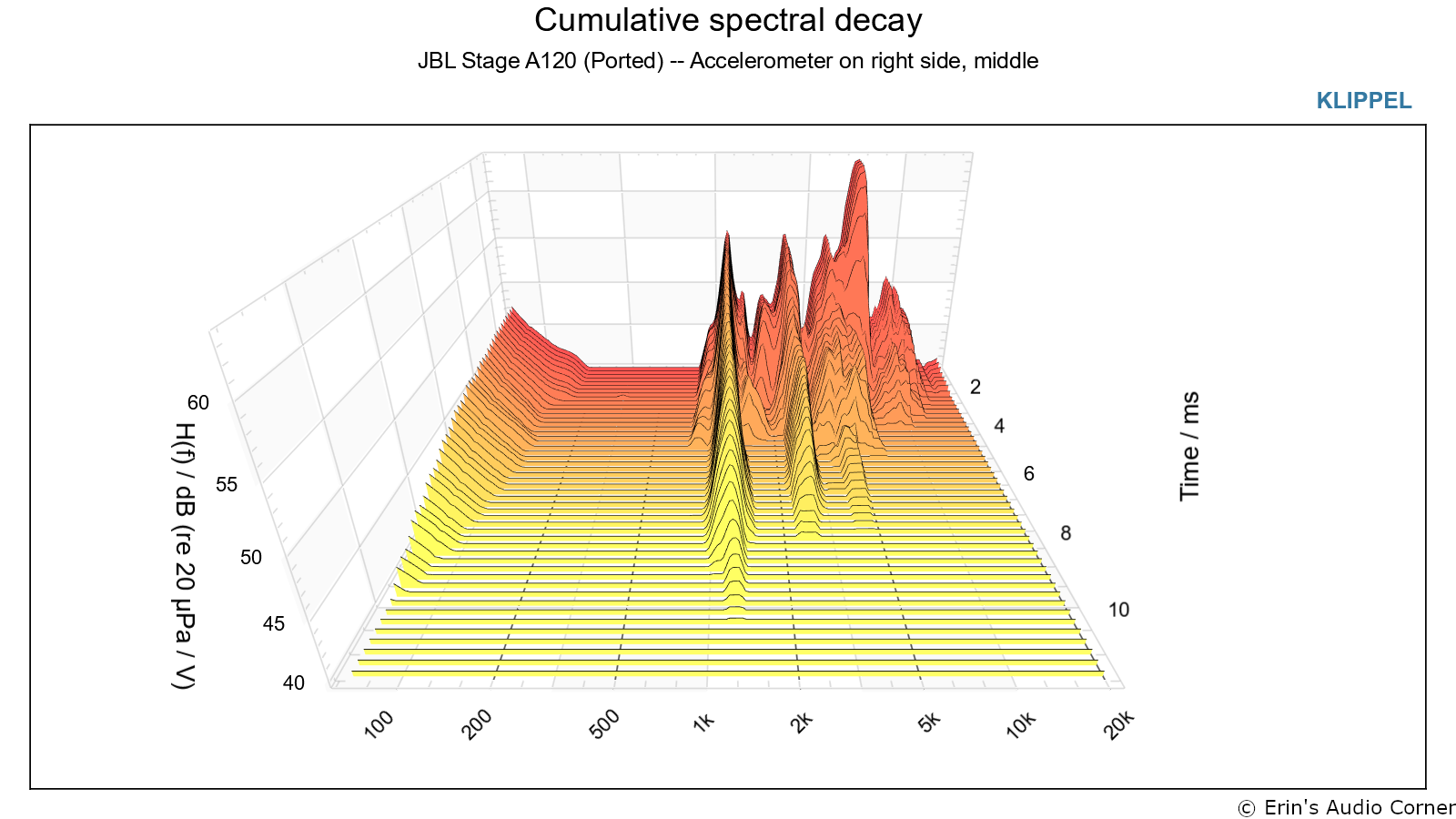
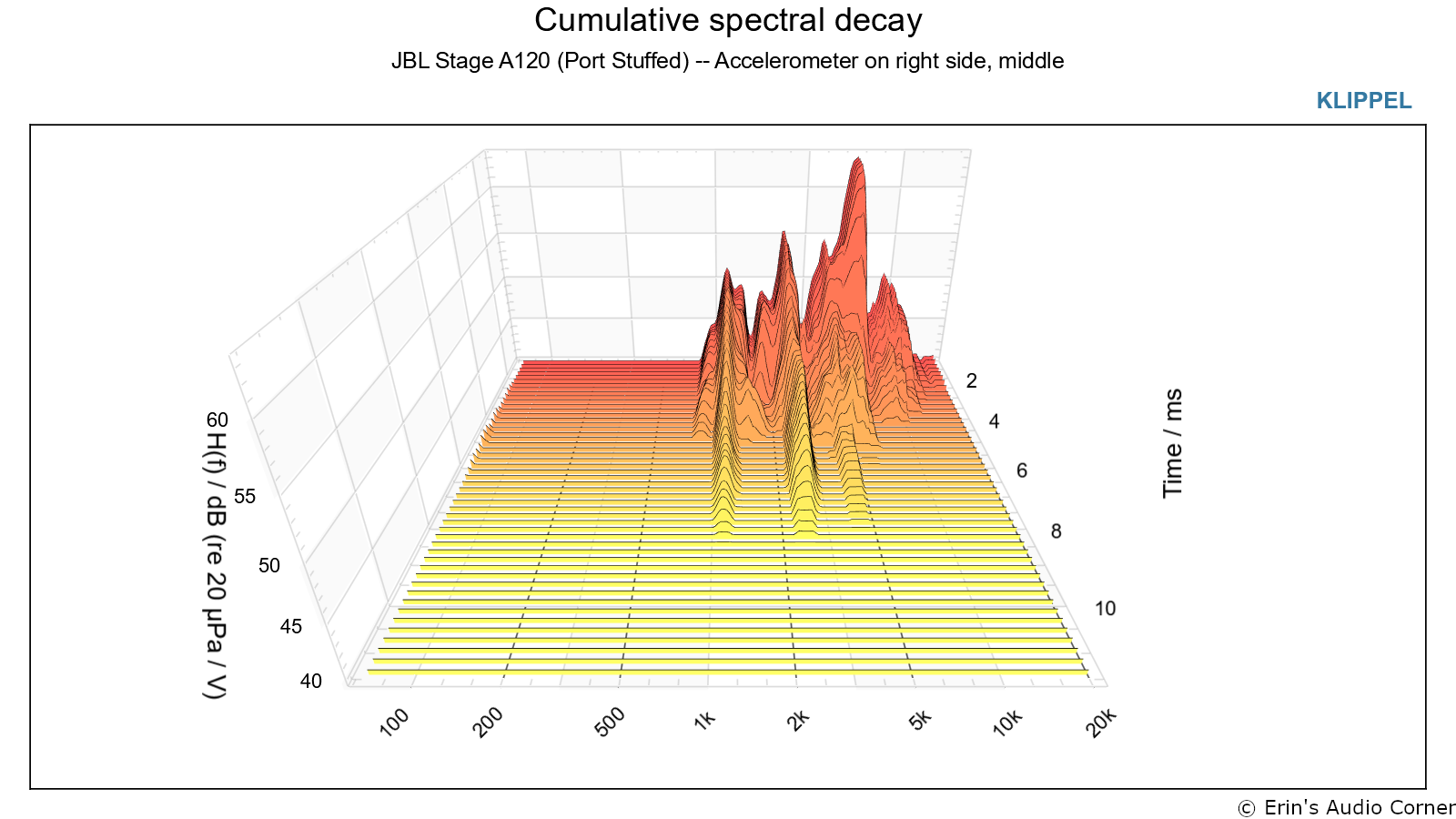
So, I then used my accelerometer to test the cabinet vibration at the side-middle and - again - see similar results. This indicates, at least to me, the directivity error in the ported configuration is attributed to the port at around 1kHz, though it is pretty marginal. What I am taking away from this data is that the enclosure itself exhibits resonance (likely due to the internal dimensions) and is causing the box to radiate sound and leak from the port resulting in the non-linearities you see in the 1-2kHz region.
Parting / Random Thoughts
If you want to see the music I use for evaluating speakers subjectively, see my Spotify playlist.
In my listening, I was really annoyed by the boomy bass and recessed midrange when listening to the speaker in the ported configuration. In sealed configuration the response was much more livable in the bass but the disparity between bass/midrange vs upper-midrange/treble was still unpleasing.
This speaker is moderately EQ-able but more so in the sealed configuration. The flat directivity between about 1.6kHz to 6kHz results in a wide soundstage if you dig that stuff. I do, but it was hard to enjoy through the recessed midrange (which, again, can be EQ’d with a shelf filter).
That said, I personally wouldn’t spend my money on these. The recently tested Emotiva Airmotiv B+ seems to me the better option. In my humble opinion.
As stated in the Foreword, this written review is purposely a cliff’s notes version. For more details about the performance (objectively and subjectively) please watch the YouTube video.
Support the Cause
If you like what you see here and want to help support the cause there are a few ways you can do so:
-
Using my Amazon affiliate link which helps me gain a small commission at no additional cost to you.
Your support helps me pay for new items to test, hardware, miscellaneous items and costs of the site’s server space and bandwidth and is very much appreciated.
You can also join my Facebook and YouTube pages if you’d like to follow along with updates.