Foreword / YouTube Video Review

The review on this website is a brief overview and summary of the objective performance of this speaker. It is not intended to be a deep dive. Moreso, this is information for those who prefer “just the facts” and prefer to have the data without the filler.

However, for those who want more - a detailed explanation of the objective performance, and my subjective evaluation (what I heard, what I liked, etc.) - please watch the below video where I go more in-depth.

Information and Photos

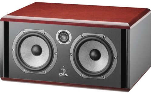
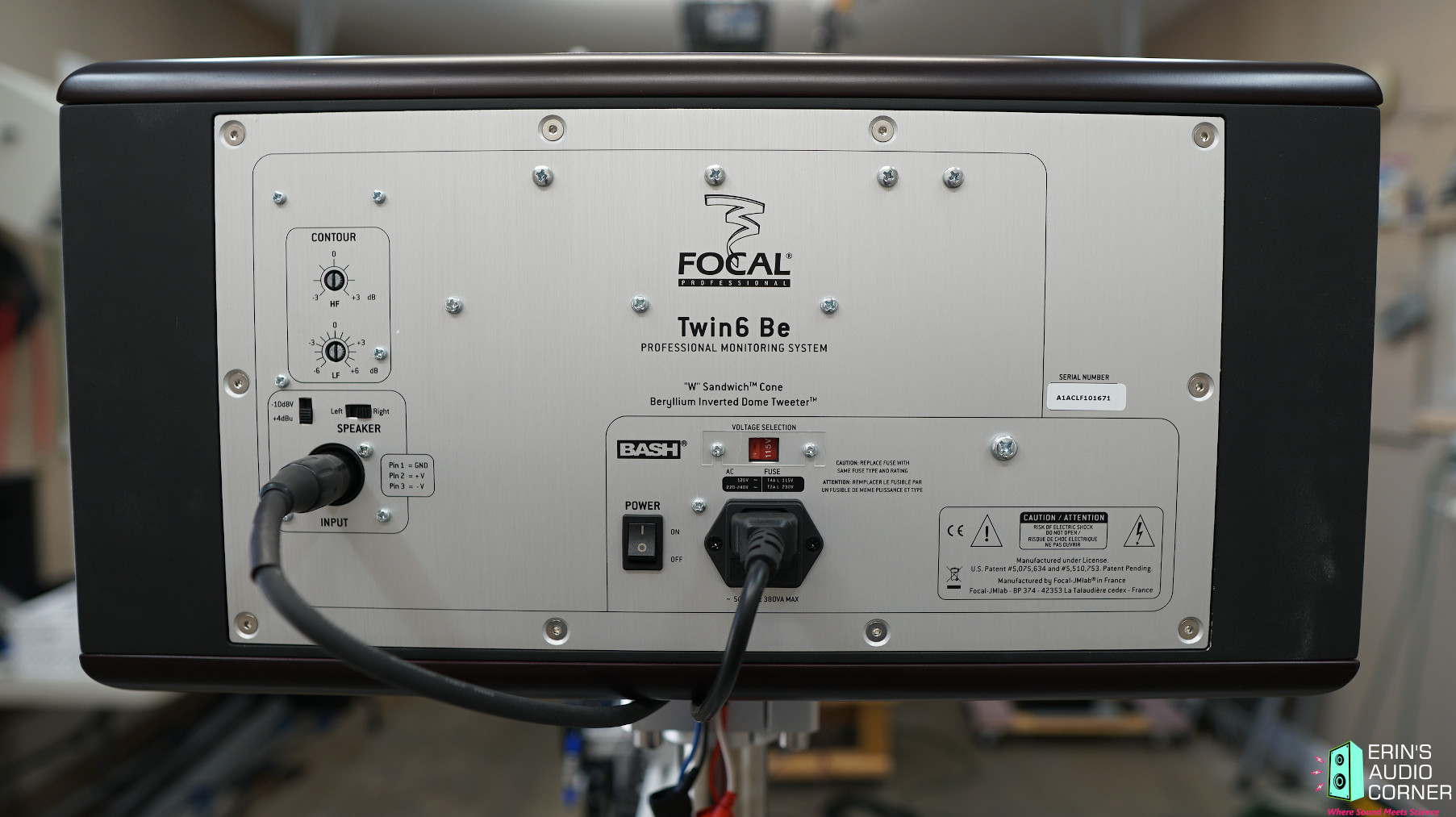
The Focal Twin6 Be is powered 2.5-way Studio Monitor. The below is from the manufacturer’s website:

The Twin6 Be is the best seller of the Focal Professional range and the most versatile work tool of the SM6 line. It represents the only necessary solution for recording, mixing and mastering. The image precision, treble definition as well as midrange neutrality are at the heart of its reputation. The excellent articulation of the bass and midbass registers, even at very high sound levels, makes it an unavoidable reference for engineers who require absolute transparency. Furthermore, the design of the Twin6 Be permits a high SPL while at the same time offering a stable tonal balance. One of the two 6.5” woofers works in large band (midrange – bass) whereas the other reproduces from 40 to 150Hz. This creates a bass that preserves all the signal dynamics, without any masking effect in the midrange, thereby keeping all its neutrality and transparency. Additional control of the bass register is accomplished by fine-tuning on the control plate on the back of the Twin6 Be in order to obtain a perfect mirror configuration with its mate. The Twin6 Be can be installed vertically or horizontally to respond to the space requirements of each studio.

MSRP for the single speaker is approximately $2200 USD and $4400 USD for a pair.

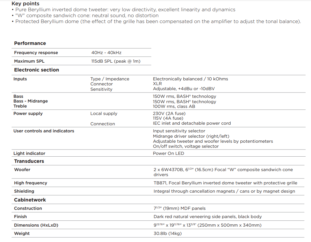
And here are some specs, again from the manufacturer’s website:

CTA-2034 (SPINORAMA) and Accompanying Data

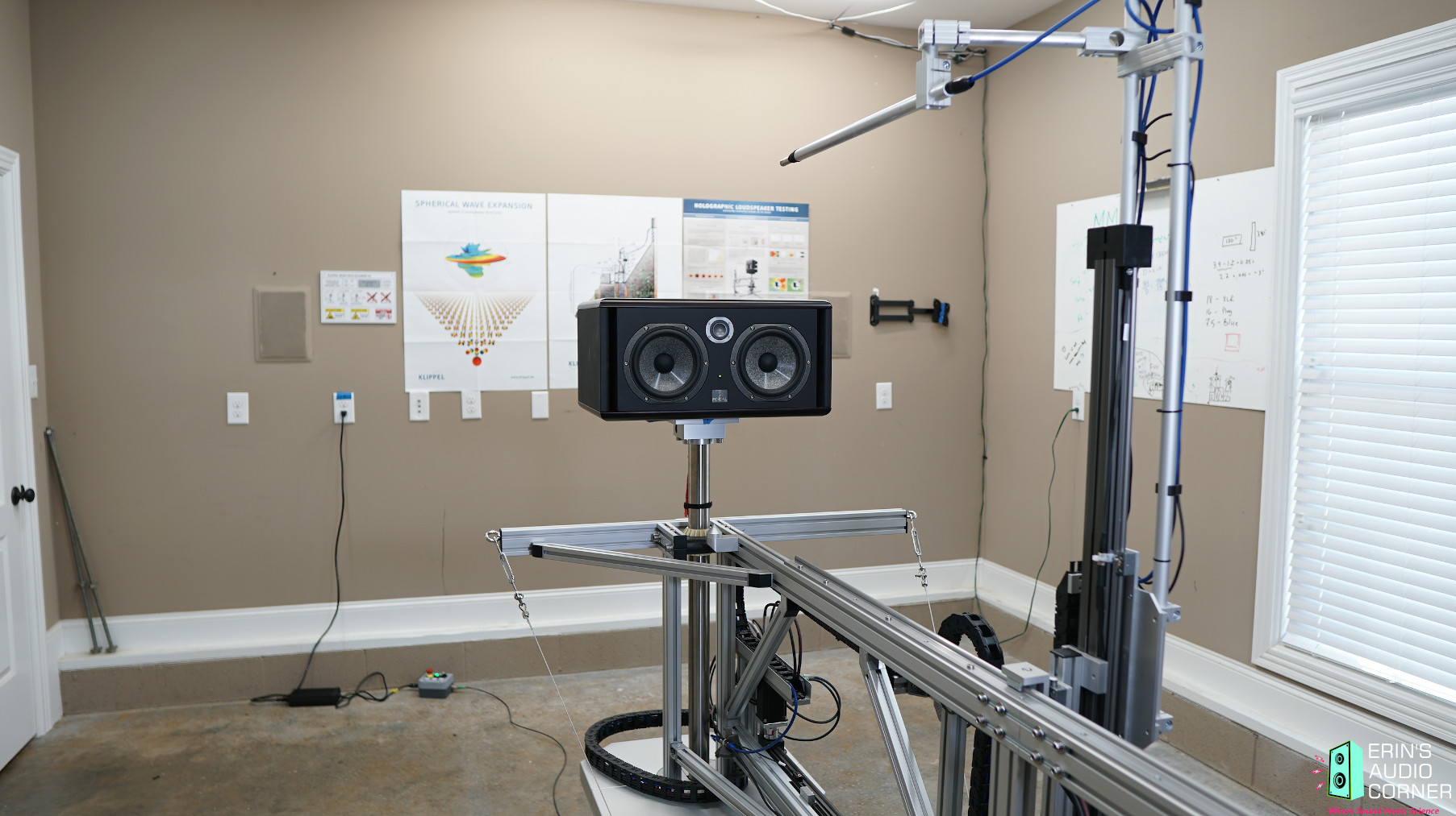
All data collected using Klippel’s Near-Field Scanner. The Near-Field-Scanner 3D (NFS) offers a fully automated acoustic measurement of direct sound radiated from the source under test. The radiated sound is determined in any desired distance and angle in the 3D space outside the scanning surface. Directivity, sound power, SPL response and many more key figures are obtained for any kind of loudspeaker and audio system in near field applications (e.g. studio monitors, mobile devices) as well as far field applications (e.g. professional audio systems). Utilizing a minimum of measurement points, a comprehensive data set is generated containing the loudspeaker’s high resolution, free field sound radiation in the near and far field. For a detailed explanation of how the NFS works and the science behind it, please watch the below discussion with designer Christian Bellmann:

A picture of the setup in my garage:

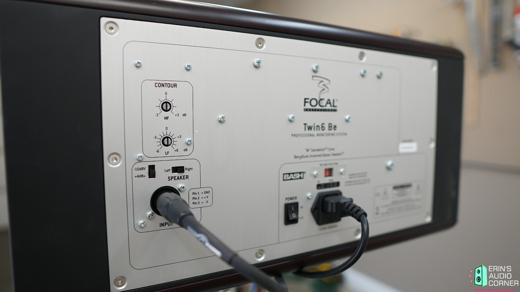
Since this speaker is atypical - due to the offset tweeter - I want to make note of how the tests (objective and subjective) were conducted. Per the manufacturer’s manual:

The Solo6 Be and Twin6 Be are designed for near field monitoring and should be placed at a distance between 1 and 3 meters from the listener, pointing towards the listening position. They can be sitting on the console top or placed on appropriate stands. In any way it is recommended that the tweeter is at a height from the floor approximately equivalent to that of the listener’s ears. If required it can make sense to place the speakers upside down so that the previous rule is better fulfilled. By design the Twin6 Be’s are rather intended for a landscape orientation, though in some situations they could be positioned vertically. As seen in the earlier rear panel description, the Twin6 Be has a switch allowing to choose which drive unit is to reproduce the mid frequencies (see below) (fig. E). Consequently it will always be possible, as desirable, to configure the speakers in a “mirror” (ie symetrical) way (fig. F). As a general rule having the “midrange” driver on the inside of the cabinet results in better imaging.

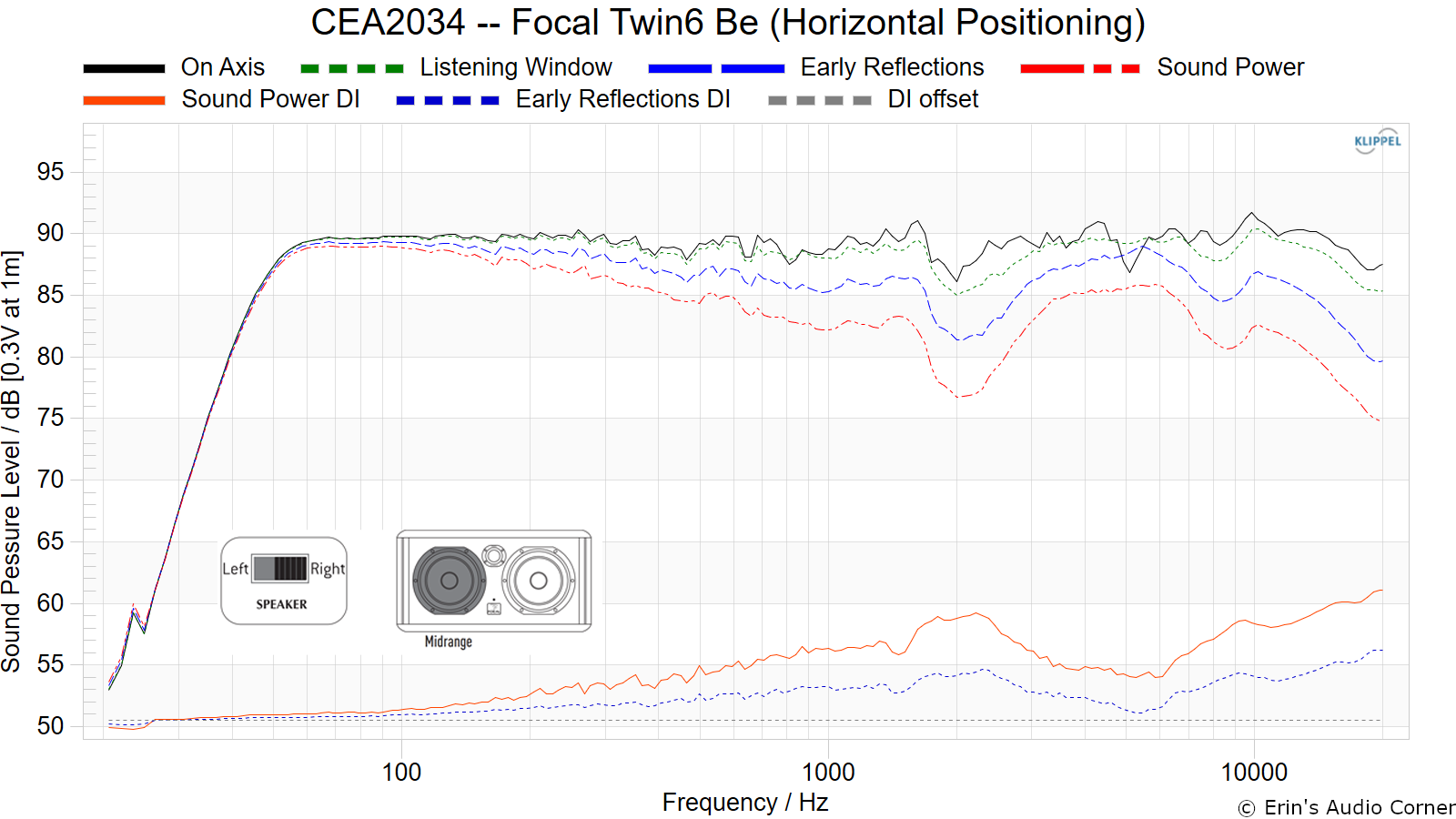
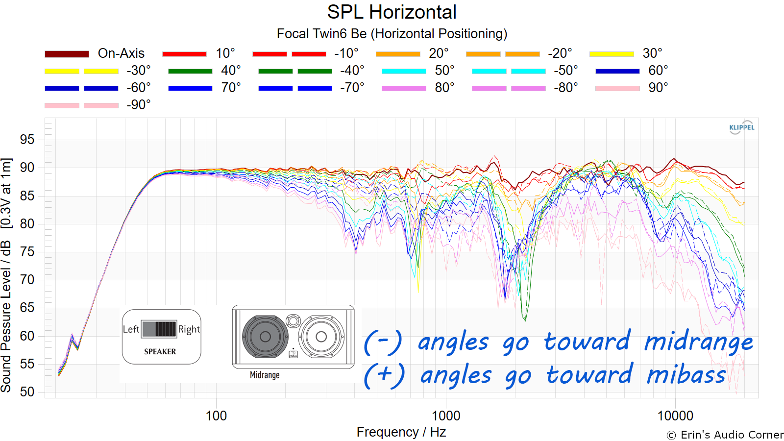
With the above in mind, this test was conducted under the following conditions: The reference plane in this test is at the tweeter. The speaker was tested in the horizontal configuration. Focal recommends the midrange be placed at the “inside” of the cabinet. This speaker was tested in the “right” configuration meaning the midrange driver is placed on the left side of the cabinet (when laying horizontally). The negative horizontal axis goes left (toward the midrange). The positive horizontal axis goes right (toward the midwoofer). I have included a graphic illustrating this configuration in the appropriate results.

Measurements are provided in a format in accordance with the Standard Method of Measurement for In-Home Loudspeakers (ANSI/CTA-2034-A R-2020). For more information, please see this link.

Note: The roll off rate of this speaker is sharp and therefore some noise was unavoidable at 25Hz which causes a spike in the response here. Ignore the response below 25Hz.

CTA-2034 / SPINORAMA:

The On-axis Frequency Response (0°) is the universal starting point and in many situations it is a fair representation of the first sound to arrive at a listener’s ears.

The Listening Window is a spatial average of the nine amplitude responses in the ±10º vertical and ±30º horizontal angular range. This encompasses those listeners who sit within a typical home theater audience, as well as those who disregard the normal rules when listening alone.

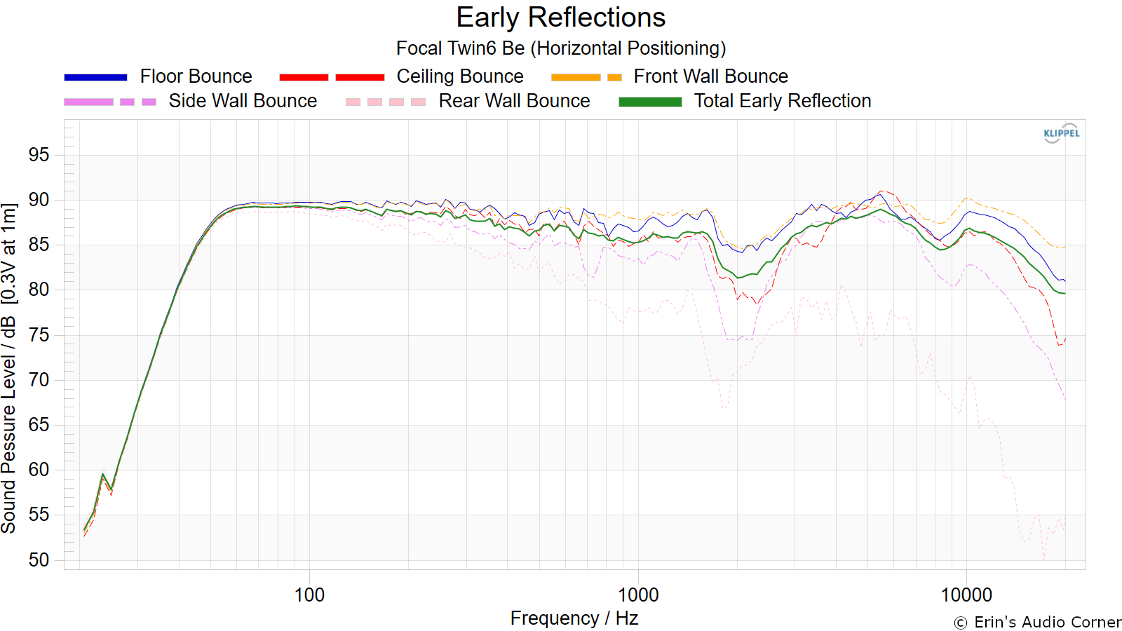
The Early Reflections curve is an estimate of all single-bounce, first-reflections, in a typical listening room.

Sound Power represents all of the sounds arriving at the listening position after any number of reflections from any direction. It is the weighted rms average of all 70 measurements, with individual measurements weighted according to the portion of the spherical surface that they represent.

Sound Power Directivity Index (SPDI): In this standard the SPDI is defined as the difference between the listening window curve and the sound power curve.

Early Reflections Directivity Index (EPDI): is defined as the difference between the listening window curve and the early reflections curve. In small rooms, early reflections figure prominently in what is measured and heard in the room so this curve may provide insights into potential sound quality.

Early Reflections Breakout:

Floor bounce: average of 20º, 30º, 40º down

Ceiling bounce: average of 40º, 50º, 60º up

Front wall bounce: average of 0º, ± 10º, ± 20º, ± 30º horizontal

Side wall bounces: average of ± 40º, ± 50º, ± 60º, ± 70º, ± 80º horizontal

Rear wall bounces: average of 180º, ± 90º horizontal

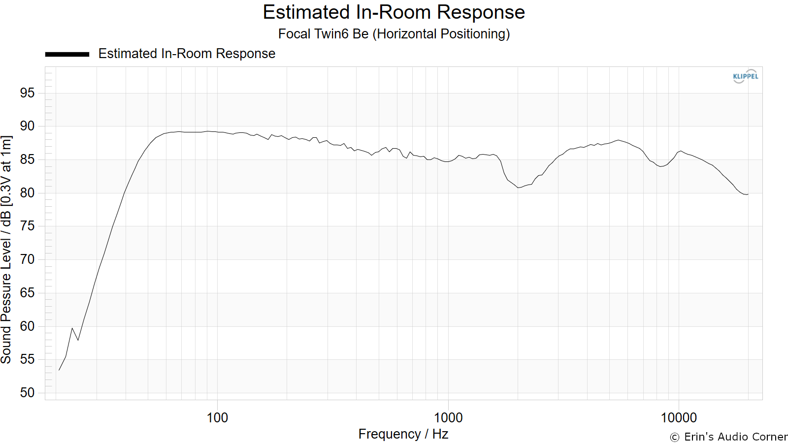
Estimated In-Room Response:

In theory, with complete 360-degree anechoic data on a loudspeaker and sufficient acoustical and geometrical data on the listening room and its layout it would be possible to estimate with good precision what would be measured by an omnidirectional microphone located in the listening area of that room. By making some simplifying assumptions about the listening space, the data set described above permits a usefully accurate preview of how a given loudspeaker might perform in a typical domestic listening room. Obviously, there are no guarantees because individual rooms can be acoustically aberrant. Sometimes rooms are excessively reflective (“live”) as happens in certain hot, humid climates, with certain styles of interior décor and in under-furnished rooms. Sometimes rooms are excessively “dead” as in other styles of décor and in some custom home theaters where acoustical treatment has been used excessively. This form of post processing is offered only as an estimate of what might happen in a domestic living space with carpet on the floor and a “normal” amount of seating, drapes, and cabinetry.

For these limited circumstances it has been found that a usefully accurate Predicted In-Room (PIR) amplitude response, also known as a “room curve” is obtained by a weighted average consisting of 12 % listening window, 44 % early reflections and 44 % sound power. At very high frequencies errors can creep in because of excessive absorption, microphone directivity, and room geometry. These discrepancies are not considered to be of great importance.

Horizontal Frequency Response (0° to ±90°):

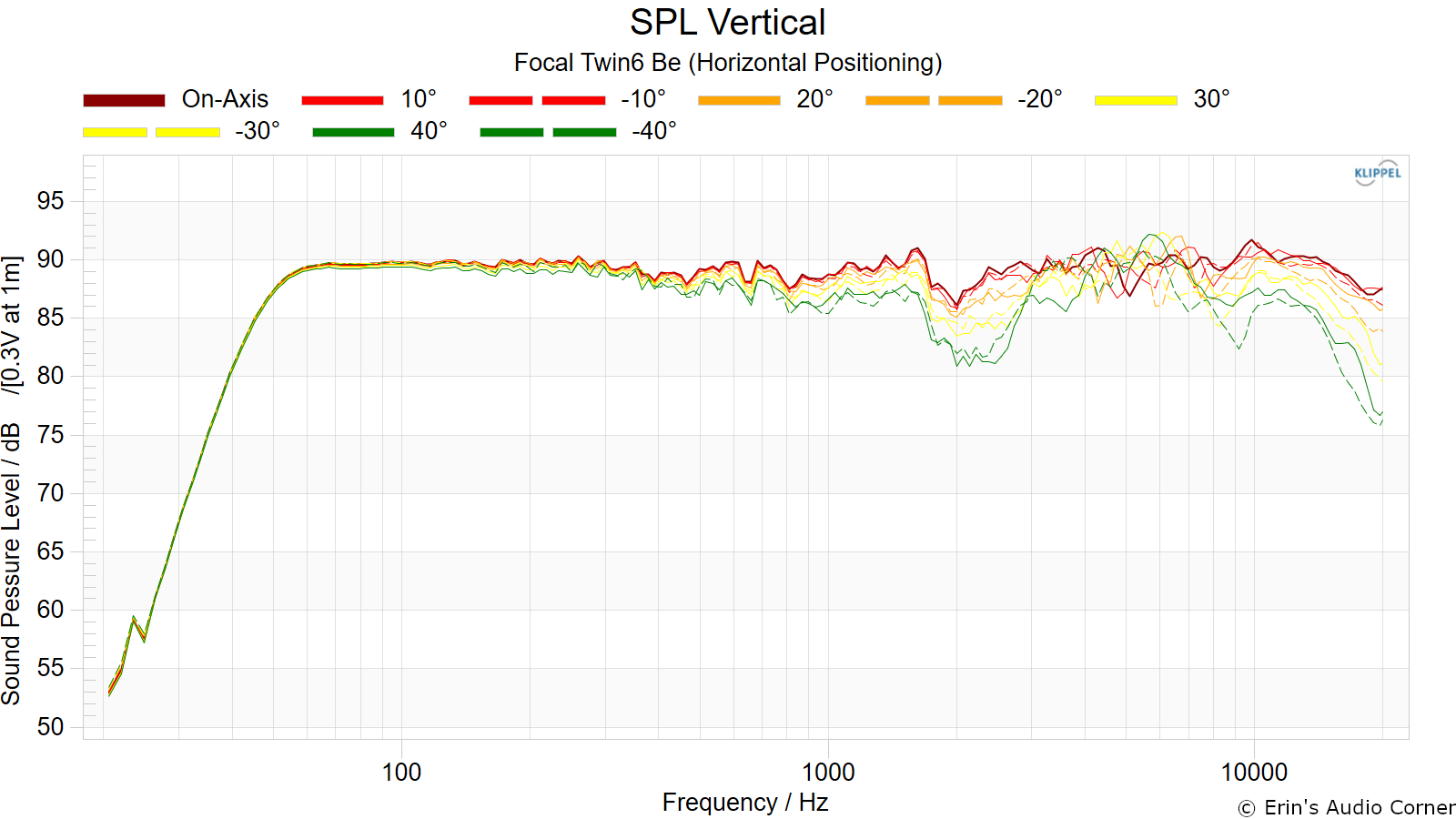
Vertical Frequency Response (0° to ±40°):

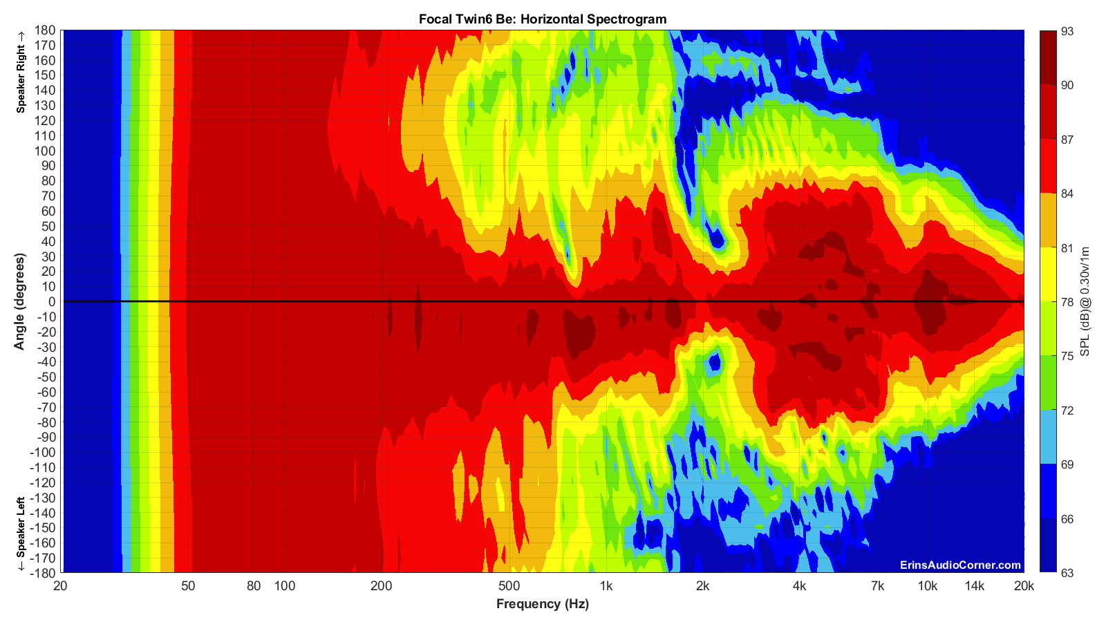
Horizontal Contour Plot (not normalized):

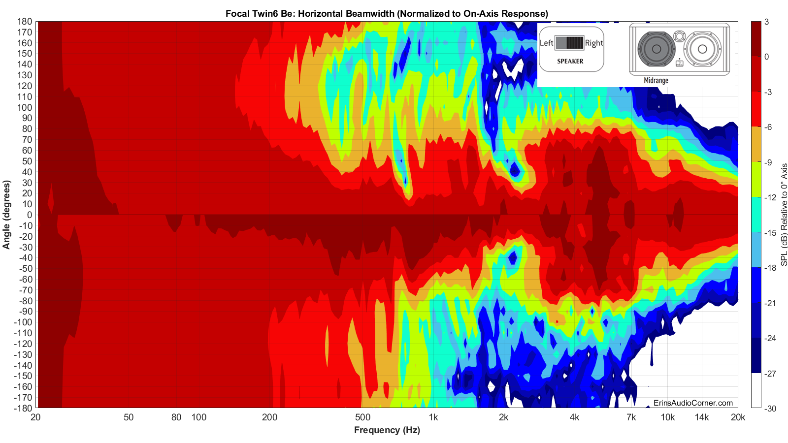
Horizontal Contour Plot (normalized):

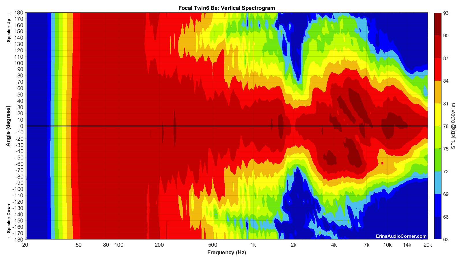
Vertical Contour Plot (not normalized):

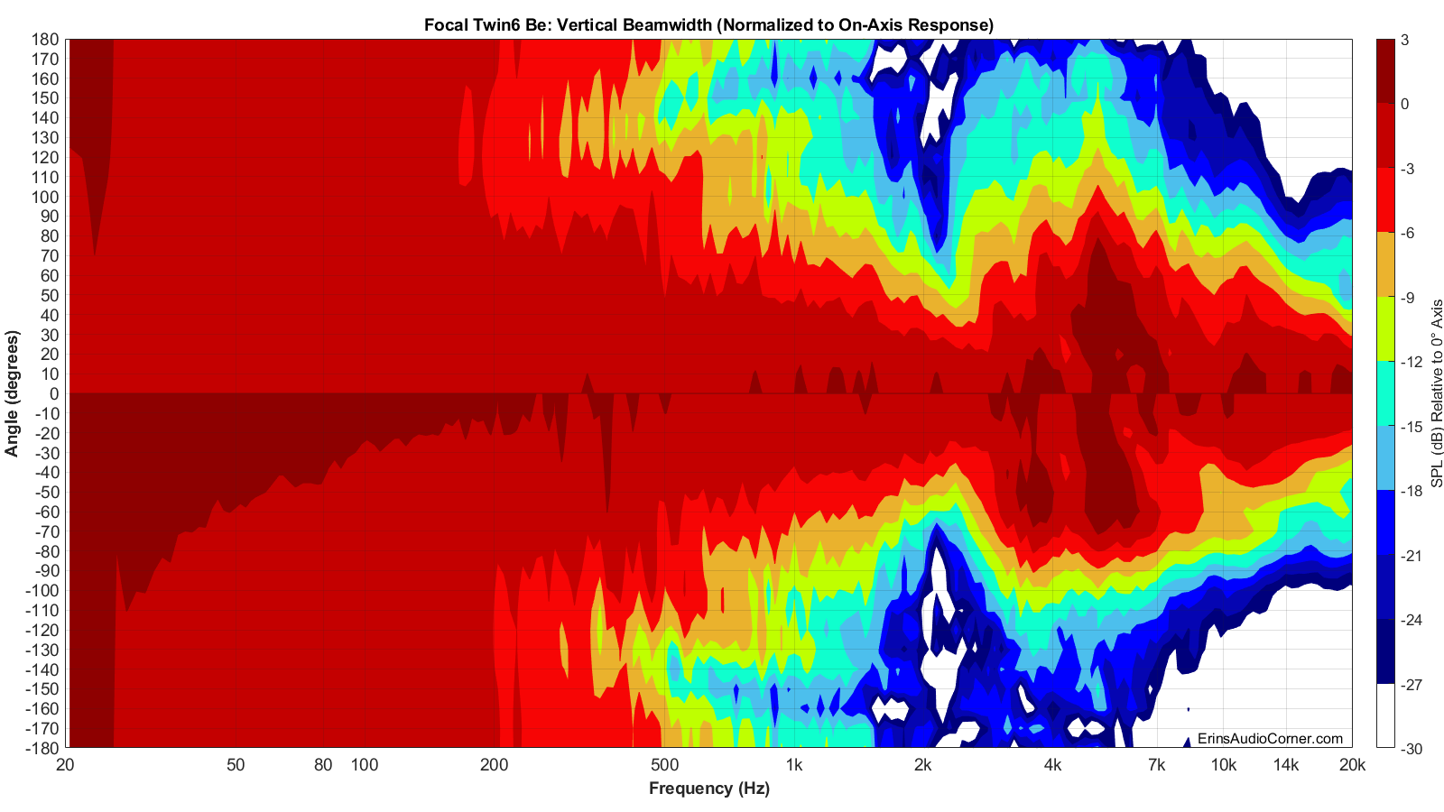
Vertical Contour Plot (normalized):

Additional Measurements

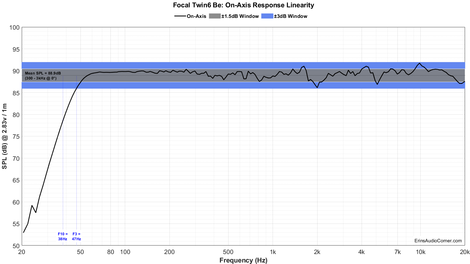
On-Axis Response Linearity

Response linearity is -2.81/+2.81 dB from 80Hz to 16kHz.

“Globe” Plots

These plots are generated from exporting the Klippel data to text files. I then process that data with my own MATLAB script to provide what you see. These are not part of any software packages and are unique to my tests.

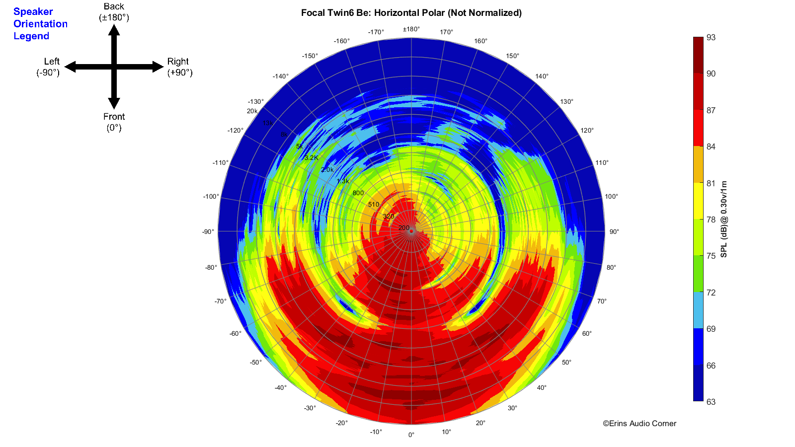
Horizontal Polar (Globe) Plot:
This represents the sound field at 2 meters - above 200Hz - per the legend in the upper left.

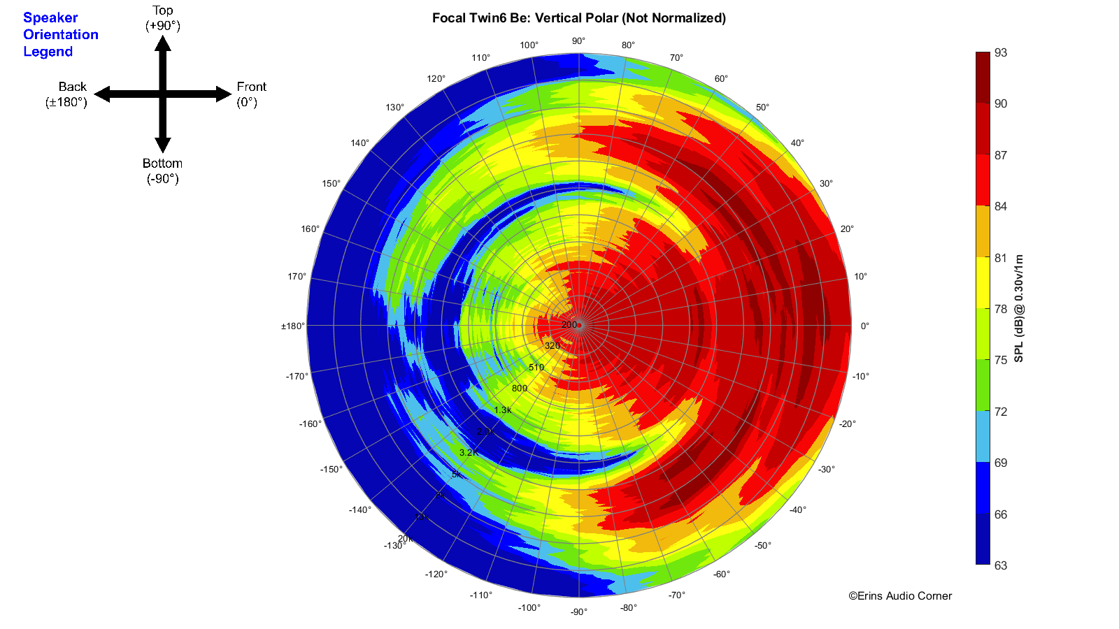
Vertical Polar (Globe) Plot:
This represents the sound field at 2 meters - above 200Hz - per the legend in the upper left.

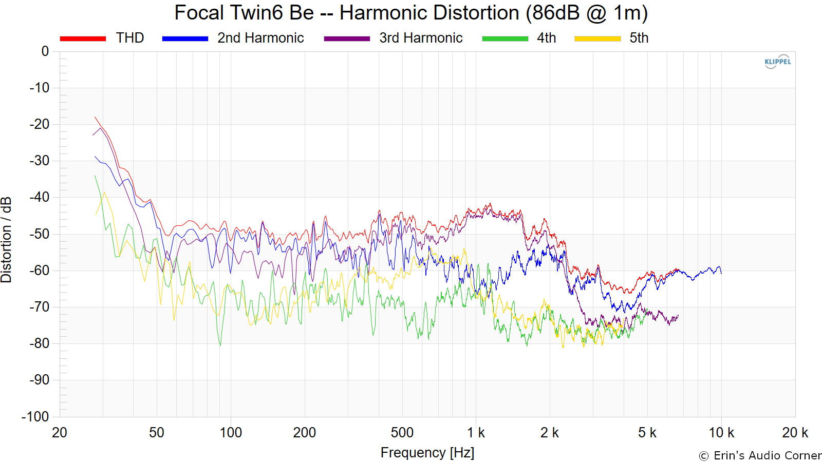
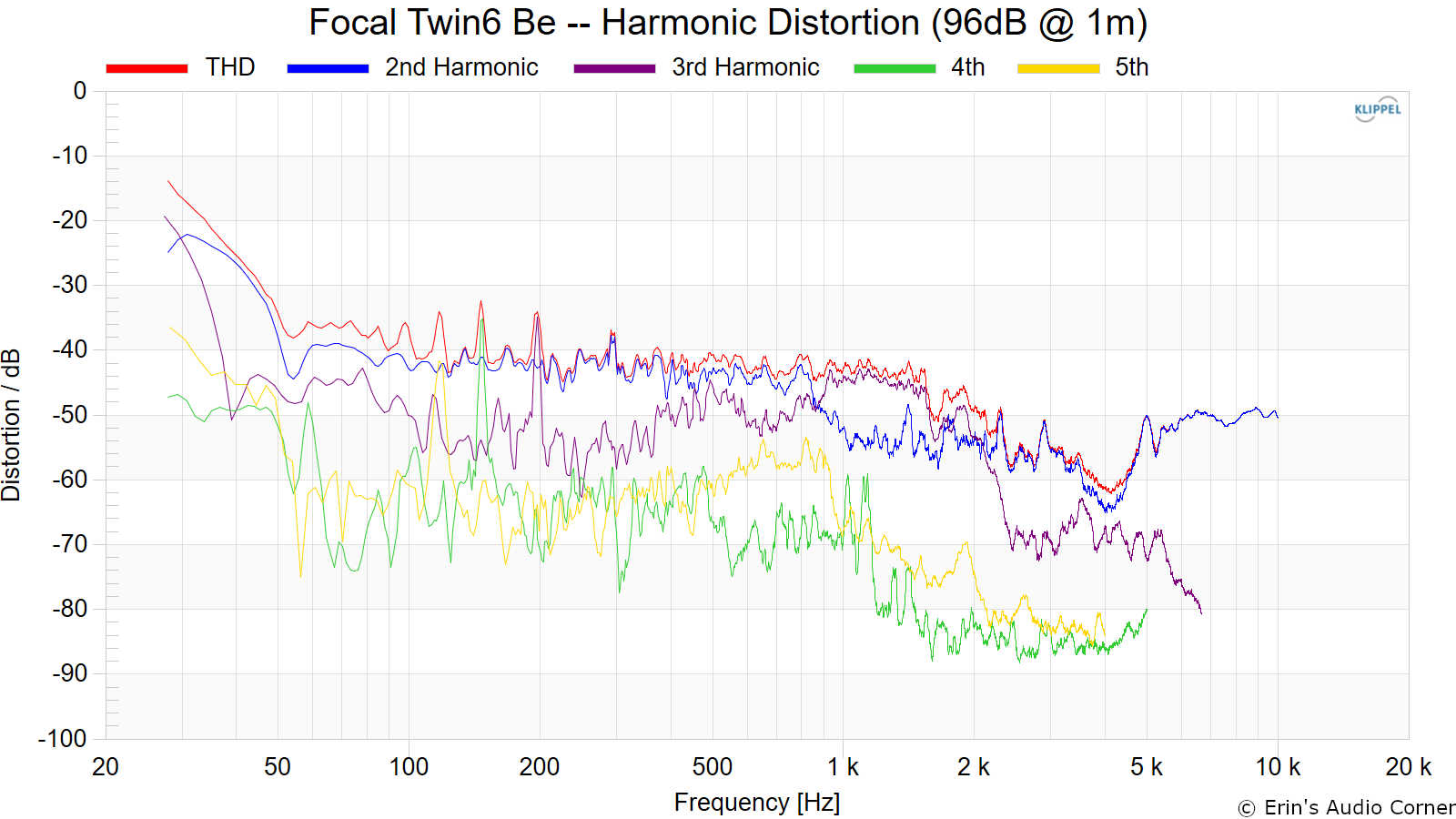
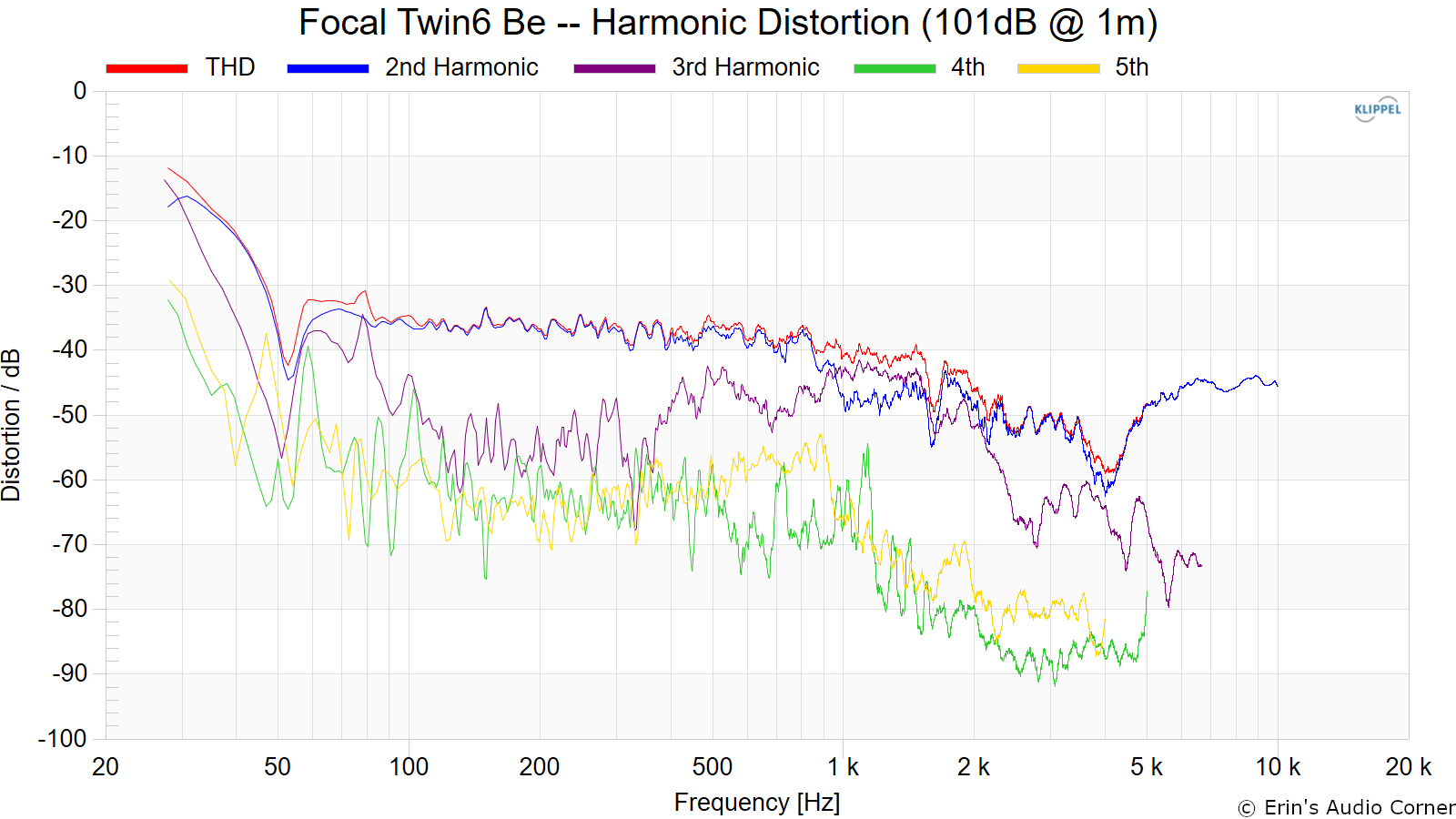
Harmonic Distortion

Harmonic Distortion at 86dB @ 1m:

Harmonic Distortion at 96dB @ 1m:

Harmonic Distortion at 101dB @ 1m:

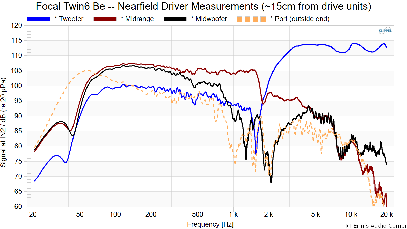
Near-Field Response

Nearfield response of individual drive units:

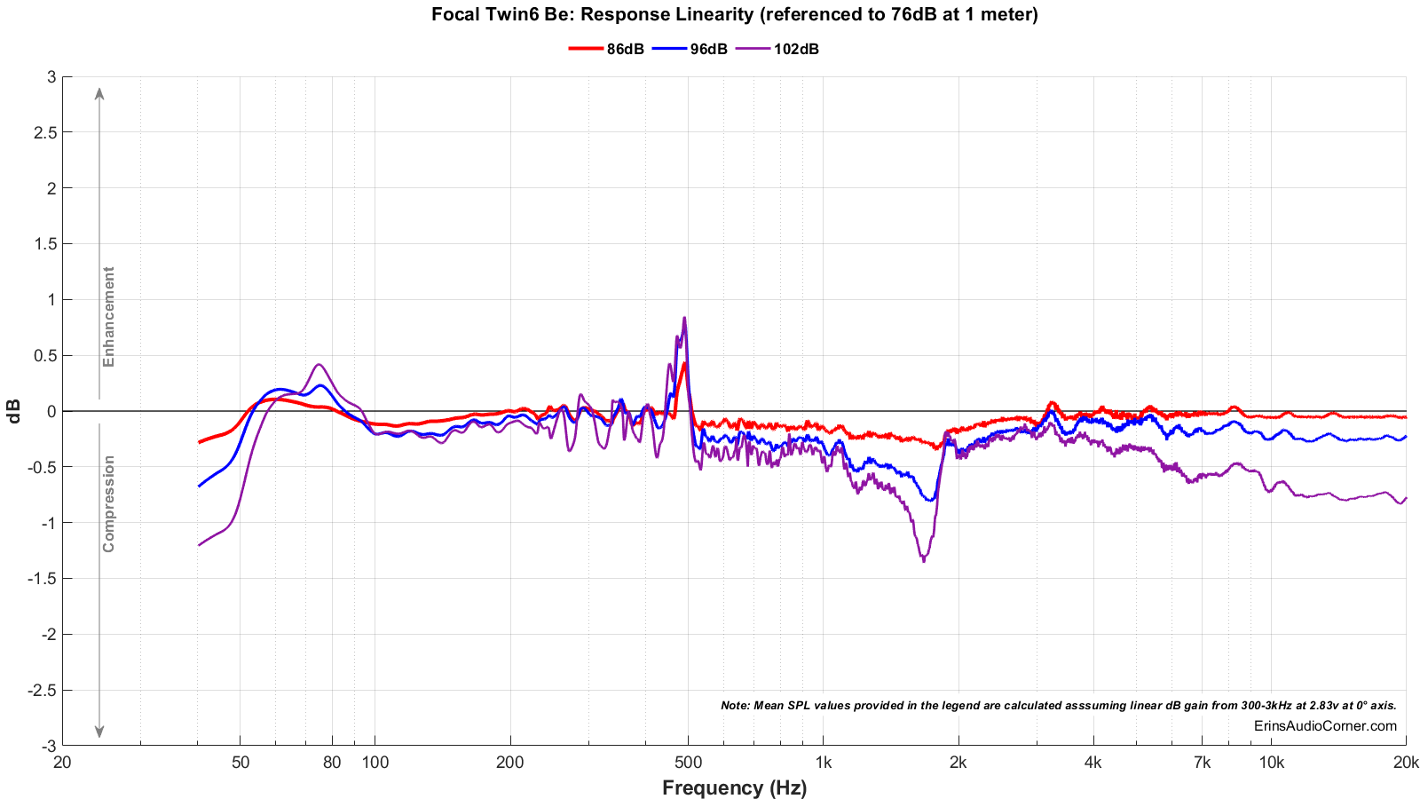
Dynamic Range (Instantaneous Compression Test)

The below graphic indicates just how much SPL is lost (compression) or gained (enhancement; usually due to distortion) when the speaker is played at higher output volumes instantly via a 2.7 second logarithmic sine sweep referenced to 76dB at 1 meter. The signals are played consecutively without any additional stimulus applied. Then normalized against the 76dB result.

The tests are conducted in this fashion:

1. 76dB at 1 meter (baseline; black)
2. 86dB at 1 meter (red)
3. 96dB at 1 meter (blue)
4. 102dB at 1 meter (purple)

The purpose of this test is to illustrate how much (if at all) the output changes as a speaker’s components temperature increases (i.e., voice coils, crossover components) instantaneously.

In-Room Measurements from the Listening Position

Below is the actual measured in-room response (with no DSP correction). This is a spatial average taken over approximately 1 cubic foot. The speakers were placed approximately 1.2m from the front wall (not the cabinets; but the actual wall). The listening position varied but stayed within the recommended 1-3 meters from the speakers.

Black = Predicted In-Room Response from SPIN data
Blue = Actual In-Room Measured Response from Main Listening Position at 1.5 meters
Purple = Actual In-Room Measured Response from Main Listening Position at 2.5 meters

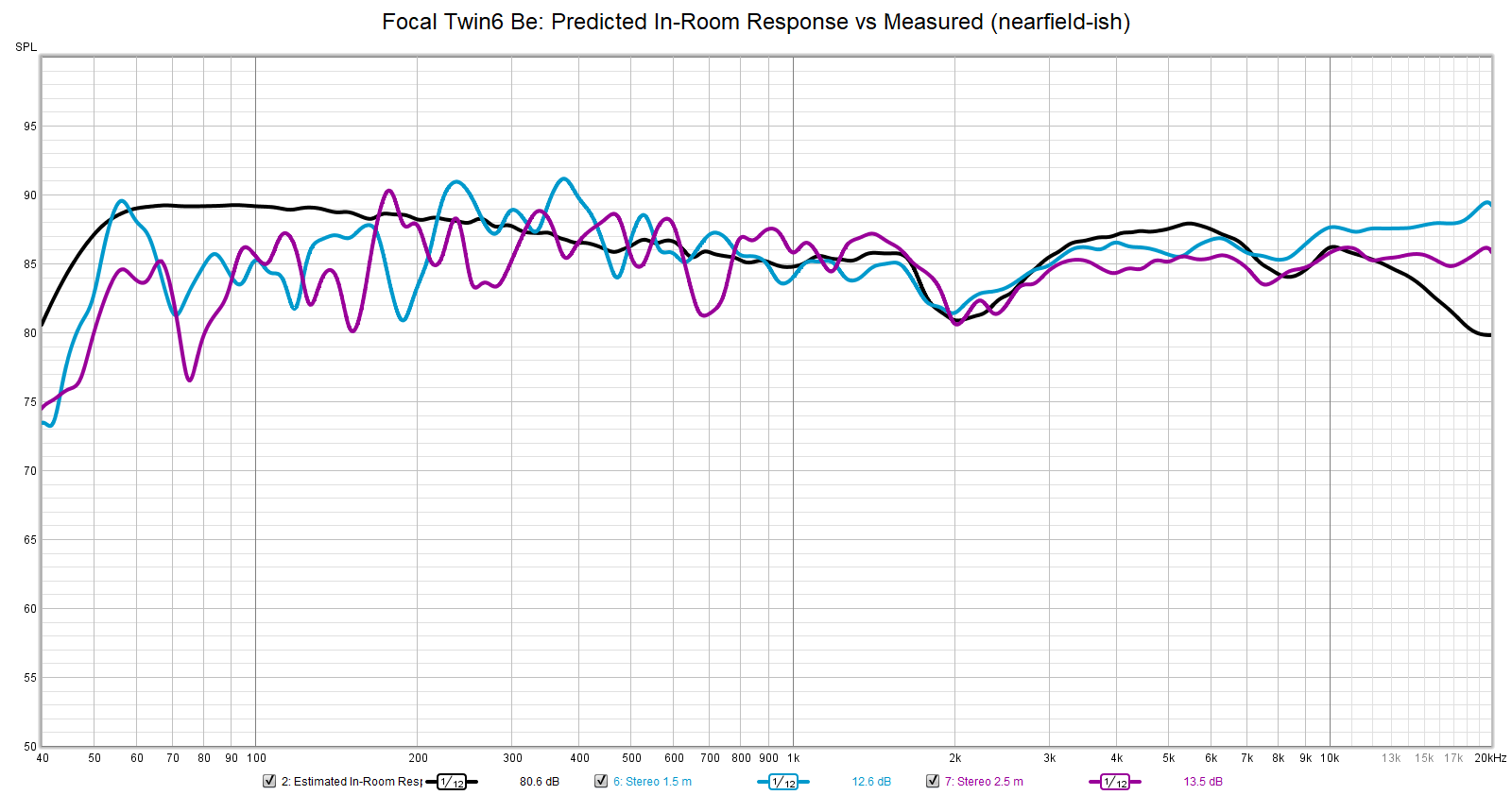
While the prediction in this test is close to the actual measured response, there is a fair bit more deviation than I typically see in my other tests. I think this is likely attributed to the fact that I measured in the nearfield (as these were designed to be listened to) in my living room. You can see in the below graphic that sitting closer to the speaker yields a higher level response in the high frequency region (blue, 1.5 meters) and when backing away (purple, 2.5 meters) the HF response comes down a bit. I think if I measured these speakers as I typically do the in-room result would have matched the prediction better. This is an example of where the speaker’s purpose (nearfield listening) should be considered when viewing data.

Tone Controls (High Frequency and Low Frequency)

These speakers come with a HF trim (±3dB) and LF trim (±6dB). I tested these and made the contours relative to 0dB as you can see in the below graphic. Basically, both sets of tone controls hinge around the 1kHz region.

Parting / Random Thoughts

If you want to see the music I use for evaluating speakers subjectively, see my Spotify playlist.

• Subjective listening was conducted at a few ranges, not exceeding 3 meters. Primarily, listening was done at about 1.5 meters. Subjective listening was conducted at 80-95dB at this distance.
• I did not try listening at different off-axis angles as this is designed to be a studio monitor and it is not reasonable that this would be listened to off-axis. So, I cannot comment on loss of fidelity as the speaker is aimed differently or the listener moves side to side.
• I did listen in both the horizontal and vertical configuration. I personally preferred the vertical configuration because I often felt I could hear the sound “pull” toward the midwoofer driver. I noticed this primarily in mono listening. When listening in stereo, this issue only arose when music was panned far left or right.
• “Soft” in the 2-3kHz region (missing some background air in Depeche Mode’s Enjoy the Silence) (missing “ck” sound of “back” in Everybody Wants to Rule the World). Miss it sometimes.
• Nice, controlled bass in Higher Love (but nothing below 50Hz to give the rumble). Great bass in Know Your Enemy.
• Excellent midbass and midrange overall!
• Great bass lines in Wrapped Around Your Finger.
• Midrange becomes “shouty” in Doo Wop at the beginning at higher volumes. This is a pretty complex track that stresses the midrange as bass if the driver also is playing deep bass. In this case, I typically chalk up such issues as IMD, though I am currently not testing IMD for loudspeakers as the requirements to do so are beyond the time I have.
• Free Fallin - incredible midrange detail.
• What Lovers Do: effects in soundstage are all on the same z-axis plane, behind the speaker’s physical placement.
• Awesome “pick” in Feel It Still.
• Until it Breaks gave me goosebumps.
• Be careful with volume. Easily get to 95dB in the nearfield without even realizing it. No distortion to signal that you need to turn it down.
• When listening in mono easily tell the midrange/midwoofer split. Not so much with stereo unless panned.
• Soundstage is about 2 feet outside of speakers and about 2 feet deep in center.
• There is zero mechanical noise from these speakers (pops, over-excursion, vent noise) even at considerable volumes.
• The on-axis response is really quite linear with the exception of the 2-3kHz dip. From the nearfield data, this seems to be due to a steep low-pass filter on the midrange. The roll off begins promptly at about 50Hz which is adequate, however, a subwoofer is obviously needed for extended bass.
• When listening, I noticed the HF tends to sound brighter the closer I was to the speaker. In the above in-room measurements you can see there is a gain of about 2dB when moving from 2.5 meters to 1.5 meters listening distance, so keep this in mind.
• Hiss: When the input sensitivity was switched to +4dBu there was no audible hiss at 1.5m and also barely noticeable with ear next to tweeter. At -10dBu hiss was noticeable from 0.5m.

I don’t have a lot of experience with dedicated monitors so I don’t want to get too excited but I have to say the midbass and midrange of these speakers is excellent. I haven’t heard such detailed midbass out of a speaker thus far. It really is incredibly impressive, dynamic and ‘sharp’ (in a good way). The highs, however, were the downside for me. I found the 2-3kHz region to be a bit “soft” which tended to make the presentation a bit “dull” as the attack of instruments just didn’t sound right. Also, I swear I heard sibilance which I would expect to see in the data around the 6-8kHz region, though, I am not seeing it. I wonder if this is simply the overall level because you can clearly see in the in-room measurements (taken nearfield) the high frequency response is tilted up the closer you are to the speaker. I did listen in the farfield at one point just to see how the overall presentation changed but I can’t honestly remember what my thoughts were about the high frequency region because I was more listening to see if the midbass and midrange got worse (they didn’t). I tried using the tone controls but - as you can see in the data - it isn’t specific enough to target just the high frequency region above 5kHz; instead the tone controls are based around 1kHz.

Is the 2kHz dip intentional? Is it a BBC dip? The midrange is cut quite steeply while the tweeter is crossed a bit higher. This could be intentional to introduce that dip. However, this seems a bit too steep for the standard BBC dip. That is what makes me think it might not be intentional. I don’t know for sure, though.

In my humble opinion, I think a couple well-implemented parametric EQ bands would take this from a “great” speaker to a “benchmark” level speaker. If you are on the fence about this speaker, I think it’s definitely worth consideration. Buy it from a reputable dealer with a liberal return policy and give it a shot.

Support the Cause

If you like what you see here and want to help support the cause you might be interested in joining my Patreon, here. You can also contribute via PayPal (the big yellow button below).

Your support helps me pay for new items to test, hardware, miscellaneous items and costs of the site’s server space and bandwidth. All of which I otherwise pay out of pocket. So, if you can help chip in a few bucks, know that it is very much appreciated.

Alternatively, if you are interested in purchasing these speakers, please consider using one of my affiliate links below. It yields me a small commission at no additional cost to you.

You can also join my Facebook and YouTube pages if you would like to follow along with updates.