Foreword / YouTube Video Review

This pair of speakers was loaned to me by Ex Machina directly for review. I was not paid or compensated in any capacity for this review.

All my reviews are done on my own time with great care to give you all the best set of data and information I can provide in order to help you make a well-informed purchase decision. I offer this for free to all who are interested. In return, if you want to support this site please see the bottom of this review for ways you can help. It is greatly appreciated.

The review on this website is a brief overview and summary of the objective performance of this speaker. It is not intended to be a deep dive. Moreso, this is information for those who prefer “just the facts” and prefer to have the data without the filler. The video below has more discussion with respect to the technical merits and subjective notes I had during my listening sessions.

< coming eventually >

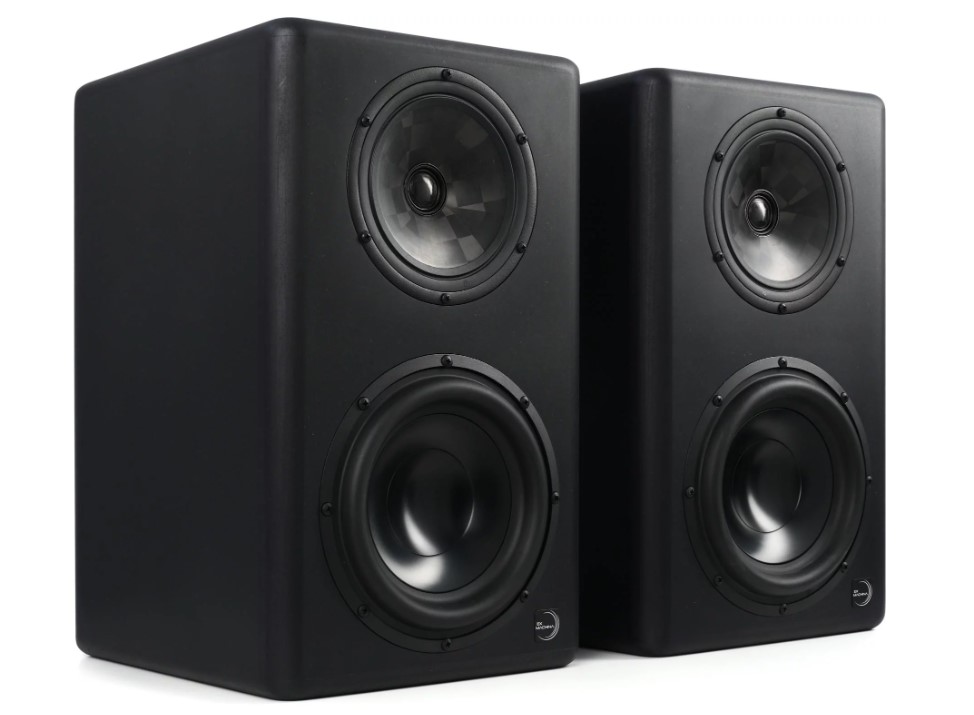
Information and Photos

Some specs from the manufacturer can be found here. Key features from the manufacturer are noted below.

COAXIAL MIDRANGE/TWEETER Mk2 Pulsar/Quasar feature a new generation of our signature coaxial midrange/tweeter drive unit. Thousands of additional R&D hours and dozens of iterations have brought a significant step forward in performance to our original design collaboration with SEAS. Below are four of the key attributes that make this one of the highest performance drivers ever made.

1. Our 25mm dome tweeters have been redesigned from the ground up using the first Composite Sound Metamodal TX™ diaphragms ever deployed. Woven from the same Textreme™ spread tow carbon fabric as our midranges, but leveraging the unique, audio specific expertise of Composite Sound, the fiber architecture and geometry of this diaphragm has been fully optimized not just for stiffness and directivity, but to actively control resonances and modes. The end result is a perfect pistonic response nearly 10khz higher than our previous 6 generation diaphragms, and such precise control of breakup that a typical driver exhibits less than .1% THD+N power average in the all critical 2-10khz midrange.
2. Our 18cm Composite Sound Metamodal TX™ midrange features iterative improvements over the original generation as well. While still a perfect piston over two octaves past its in use frequency range, we have now optimized the ratio of radial to circumferential stiffness to further improve off-axis behavior as we approach our 2khz crossover. The diaphragm is still precisely shaped to behave as an optimized waveguide for the concentric tweeter, and the newly designed geometry of the tweeter diaphragm has been further optimized to load this waveguide.
3. The thin-lip, fully underhung surround all but eliminates the on-axis suckout and phase cancellation issues that plague most coaxial drive units.
4. The advanced neodymium motor structure and high performance spider have been further augmented with a new copper shorting sleeve to lower high frequency inductance, resulting in even lower distortion than our first generation drive units.

SUBWOOFER

• Both Pulsar and Quasar feature the same SEAS designed and built 22cm subwoofer drive units. High performance, long-throw suspension systems and fully FEA optimized magnetic gaps and motor architectures give these subwoofers 28mm of linear peak to peak excursion and 56mm before damage. Combined with an ultra low resonant frequency of 24hz and pistonic linearity all the way up to 1.2khz, they provide our loudspeakers with extraordinary low end power, extension and precision.

CABINET

• All our loudspeakers feature highly braced, sealed cabinets, which completely eliminate the group delay, air compression and chuffing that plague most traditional ported loudspeakers. They are made from a combination of 19mm and 30mm thick Valchromat: a much stiffer, denser and better damped material than the traditional MDF. This makes our cabinets highly inert and non-resonant, all but eliminating destructive coupling to the pistonic output of the drive units.

AMPLIFIERS

• All our loudspeakers employ second generation Hypex Ncore amplifier modules, which combine high efficiency with ultra-low distortion and output impedance. Each drive unit is powered by its own dedicated amplifier, with 100 watts available to the midrange, 50 watts available to the tweeter on Pulsar and 75 watts available on Quasar, and 250 watts available to each subwoofer.

DSP & CONVERSION

• The final, “secret sauce” of our loudspeakers is our proprietary, in-house DSP deployment and calibration technology, which MkII improves even further. Each loudspeaker now features a 7 dedicated 5th generation SHARC+ DSP, providing 4x the computing power of our previous generation, as well as flagship AKM AK4493 and AK5572 based discrete conversion. As the final step in production, a unique, serial number specific measurement and calibration is applied to each loudspeaker, linearizing the frequency response to +/- 1db, and the phase response to +/- 15° across the entire specified range. This in turn means that any two speakers of a given model will always act as a matched pair. Finally, the newly available compute headroom has allowed us to improve the precision of our calibration code to a point where our loudspeakers can accurately reproduce square wave and single cycle impulses, even at the crossovers.

As of this writeup, the price per pair is approximately $11,699 USD.

CTA-2034 (SPINORAMA) and Accompanying Data

All data collected using Klippel’s Near-Field Scanner. The Near-Field-Scanner 3D (NFS) offers a fully automated acoustic measurement of direct sound radiated from the source under test. The radiated sound is determined in any desired distance and angle in the 3D space outside the scanning surface. Directivity, sound power, SPL response and many more key figures are obtained for any kind of loudspeaker and audio system in near field applications (e.g. studio monitors, mobile devices) as well as far field applications (e.g. professional audio systems). Utilizing a minimum of measurement points, a comprehensive data set is generated containing the loudspeaker’s high resolution, free field sound radiation in the near and far field. For a detailed explanation of how the NFS works and the science behind it, please watch the below discussion with designer Christian Bellmann:

Measurements are provided in a format in accordance with the Standard Method of Measurement for In-Home Loudspeakers (ANSI/CTA-2034-A R-2020). For more information, please see this link.

The reference plane is at the tweeter and I have provided both the on-axis (0°) as well as 10° horizontal response (typically, coaxial drivers are best listened to slightly off-axis; this speaker is no different in that regard). For this reason, only the initial CEA-2034 measurement is provided with 0°. All subsequent measurements are referenced to 10° as is the second CEA-2034 result.

Note: For full disclosure, I tested this speaker twice. My initial CTA-2034 results did not reflect what Ex Machina expected per their own measurements. I contacted Ex Machina to let them know. This is something I do on an “as needed” basis; usually when I feel the manufacturer has provided due diligence to publishing data and/or their measurement process and something, somewhere between our two methods is so fundamentally different that it is worthwhile to discuss before measurements are published. Ultimately, I sent the speakers back, they provided a firmware update and returned the speakers to me. However, the results still did not reflect what they expected so further discourse continued. It was concluded that the reference point in my measurements was the primary difference. As per all my measurements (unless otherwise noted), I provided results on the design axis at 2 meters distance. Ex Machina was very explicit that their reference point for this speaker is in the nearfield which is at approximately 0.20-0.50 meters. So, I have provided both my standard set of data in addition to nearfield measurements per their request.

This is the first time I have come across such a difference in what the manufacturer expects in their response vs what I get (regardless of how close in the nearfield or farfield the measurements are taken; as long as proper summation of the drivers are achieved). Frankly, this is an outlier case and rather than argue one side or the other I have provided a portion of Ex Machina’s email below for further clarification from their end. To be honest, it doesn’t jive with my experience but I feel it would be unfair to not at least give them the benefit of the doubt in this particular case and I therefore have provided my own nearfield measurements at varying distances (0.20 meters to 0.50 meters, off-axis at 10°) which matches what they recommend. You can see that while the response at their recommendation is more linear than the response at the standard 2m distance, it is not as linear as was expected. Again, I point you to their own rationale provided below (a snippet of our latest correspondence and mine following). I want to thank Ex Machina for their willingness to share their measurements/process in order to come to an understanding on said differences.

Ex Machina’s reply:

Importantly, this identifies a fundamental disconnect between the NFS approach to speaker characterization and the intent of our speaker design and calibration. While there is always going to be a shift in the frequency balance of acoustic energy at different listening/measurement positions, we calibrate on the plane of the tweeter with the expectation that the user will be at a listening position that is on or above that plane. This is in keeping with typical usage scenarios. As such, the magnitude response that is estimated and/or aggregated from a multitude of measurements that extend equally above and below the tweeter plane, while a meaningful characterization of the behavior of the speaker as a spherical source of sound, does not produce an appropriate characterization of the behavior and listening experience of the Pulsar in its intended operating context. In other words, the DSP calibration is, by design, correcting for the subwoofer’s output within the listening “cone” (technically half-cone) and not the output in front of or below the subwoofer. This was mentioned in a previous email, but we didn’t extrapolate clearly (apologies for that). The point is, you can say you are seeing a single symptom -increased LF- born of two different interactions with the same mechanism. Neither of which we correct for, otherwise, when in our cone/recommended listening position, there would be too little LF. This is further corroborated by your measurements of the individual drivers taken directly in front of each driver. At the same voltage input, the subwoofer is outputting more energy directly in front of it when compared to the energy in front of the coaxial. However, this energy integrates with the output from the coaxial to produce the perceived/received magnitude response within the region above the plane of the tweeter, which is the intended target of the DSP correction. As you can imagine, if the subwoofer were outputting the same energy directly in front of it as the coaxial then the integrated field within the listening region would be light on bass energy. The central point here is that your measurements are accurate for the way, and things, you are measuring, but simultaneously, so are ours. Ours are meant to capture the response/performance of the isolated speaker within the intended listening position, and given the way we are correcting this is information that naturally will not be available to the Klippel system. We do not correct for anything else. If you wanted to recreate ours, you could easily do so by measuring a single (or multiple at the same position) full frequency sweep, tweeter 1m from the ground, at tweeter height, 10deg horizontal off axis. You got close by taking a singe measurement of the drivers individually, but you moved the mic to each driver. Next time, simply keep it aimed at the recommended cal position and run the full sweep. This would naturally undo the benefit of NFS. Although, if it isn’t too terrible, you could simply do it outside (I know its hhhhhhooooootttt) so this is isn’t exactly appealing. So its completely understood if you don’t, but the point is our measurements can be recreated/repeated and unfortunately can’t be extrapolated by nature of the difference between how we measure, (and subsequently calibrate), and how Klippel measures. I hope this clarifies our measurement methodology and how/why it differs from yours. We would be happy to discuss any details that remain unclear, either for your review or as a fun academic investigation for your own edification. We appreciate your diligence and patience with us and look forward to your review.

My reply:

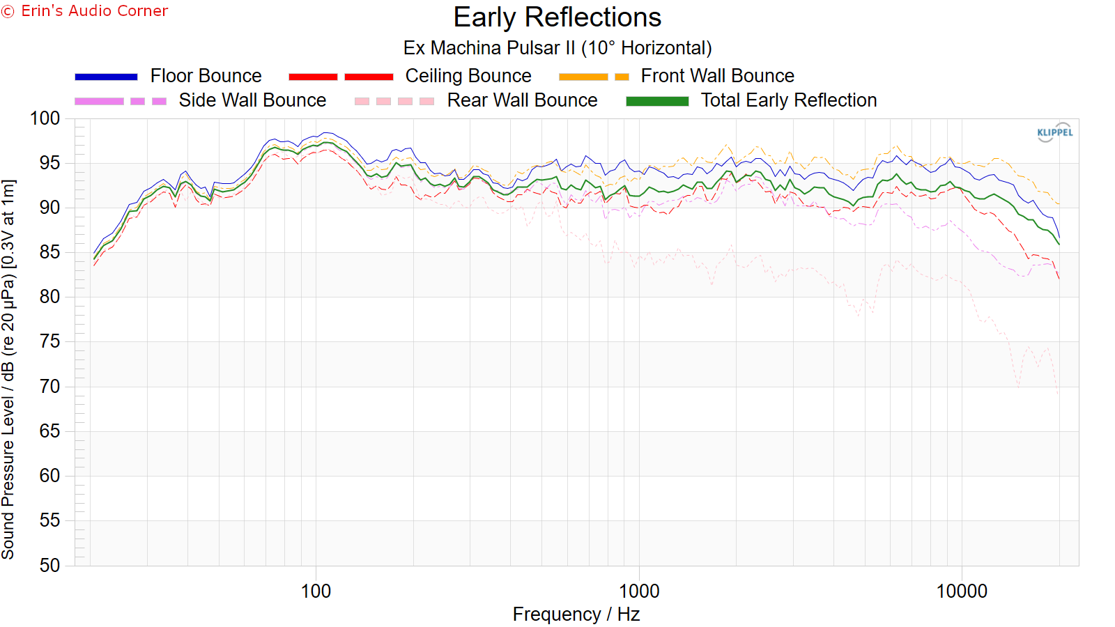
Thanks for the information. I’m extremely swamped right now but I did read through it. I was hoping to see an outdoor GP measurement that has resolution down to 20Hz because - as you noted - the indoor measurements are influenced by the room in the area I am particularly interested in discussing with you: the response below 200Hz. But I understand if you don’t care to spend any additional time on this. And your other measurements corroborate what I am seeing in mine (as you already noted). I put the speaker back on the test stand and performed a gated measurement per your suggestion. 0.20 meters, tweeter about 6 feet off the ground, microphone at tweeter level, 10 degrees off-axis. I measured it at three distances:

• 0.20 meters (red)
• 0.30 meters (blue)
• 0.50 meters (black) (obviously, there is some reflection that shows up at the furthest distance)
  
  I tried my best to match the SPL. What I see here is what you were telling me: there is a clear difference in the bass level as you move near/away from the woofer. From this, indeed, we can see the level seems at the sweet spot around 0.30 meters. I am still perplexed at the dip ~50Hz which also shows up in your datasets. It’s there in all my measurements: NFS, outdoor ground plane and now gated measurements. As well as yours.

That’s pretty much it. I thank Ex Machina for their willingness to resolve the discrepancy and I stand by my results as they are provided in this review.

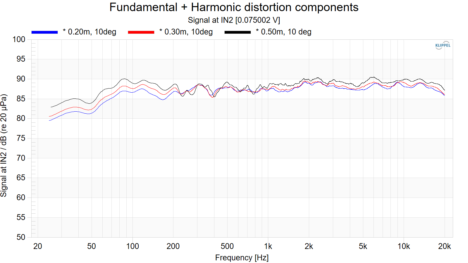
CTA-2034 / SPINORAMA:

The On-axis Frequency Response (0°) is the universal starting point and in many situations it is a fair representation of the first sound to arrive at a listener’s ears.

The Listening Window is a spatial average of the nine amplitude responses in the ±10º vertical and ±30º horizontal angular range. This encompasses those listeners who sit within a typical home theater audience, as well as those who disregard the normal rules when listening alone.

The Early Reflections curve is an estimate of all single-bounce, first-reflections, in a typical listening room.

Sound Power represents all of the sounds arriving at the listening position after any number of reflections from any direction. It is the weighted rms average of all 70 measurements, with individual measurements weighted according to the portion of the spherical surface that they represent.

Sound Power Directivity Index (SPDI): In this standard the SPDI is defined as the difference between the listening window curve and the sound power curve.

Early Reflections Directivity Index (EPDI): is defined as the difference between the listening window curve and the early reflections curve. In small rooms, early reflections figure prominently in what is measured and heard in the room so this curve may provide insights into potential sound quality.

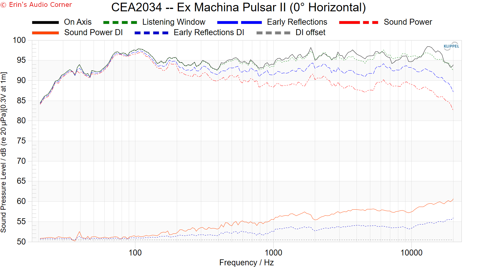
Early Reflections Breakout:

Floor bounce: average of 20º, 30º, 40º down

Ceiling bounce: average of 40º, 50º, 60º up

Front wall bounce: average of 0º, ± 10º, ± 20º, ± 30º horizontal

Side wall bounces: average of ± 40º, ± 50º, ± 60º, ± 70º, ± 80º horizontal

Rear wall bounces: average of 180º, ± 90º horizontal

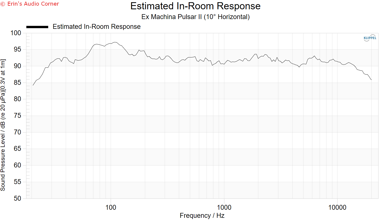
Estimated In-Room Response:

In theory, with complete 360-degree anechoic data on a loudspeaker and sufficient acoustical and geometrical data on the listening room and its layout it would be possible to estimate with good precision what would be measured by an omnidirectional microphone located in the listening area of that room. By making some simplifying assumptions about the listening space, the data set described above permits a usefully accurate preview of how a given loudspeaker might perform in a typical domestic listening room. Obviously, there are no guarantees, because individual rooms can be acoustically aberrant. Sometimes rooms are excessively reflective (“live”) as happens in certain hot, humid climates, with certain styles of interior décor and in under-furnished rooms. Sometimes rooms are excessively “dead” as in other styles of décor and in some custom home theaters where acoustical treatment has been used excessively. This form of post processing is offered only as an estimate of what might happen in a domestic living space with carpet on the floor and a “normal” amount of seating, drapes and cabinetry.

For these limited circumstances it has been found that a usefully accurate Predicted In-Room (PIR) amplitude response, also known as a “room curve” is obtained by a weighted average consisting of 12 % listening window, 44 % early reflections and 44 % sound power. At very high frequencies errors can creep in because of excessive absorption, microphone directivity, and room geometry. These discrepancies are not considered to be of great importance.

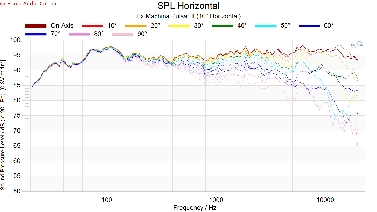
Horizontal Frequency Response (0° to ±90°):

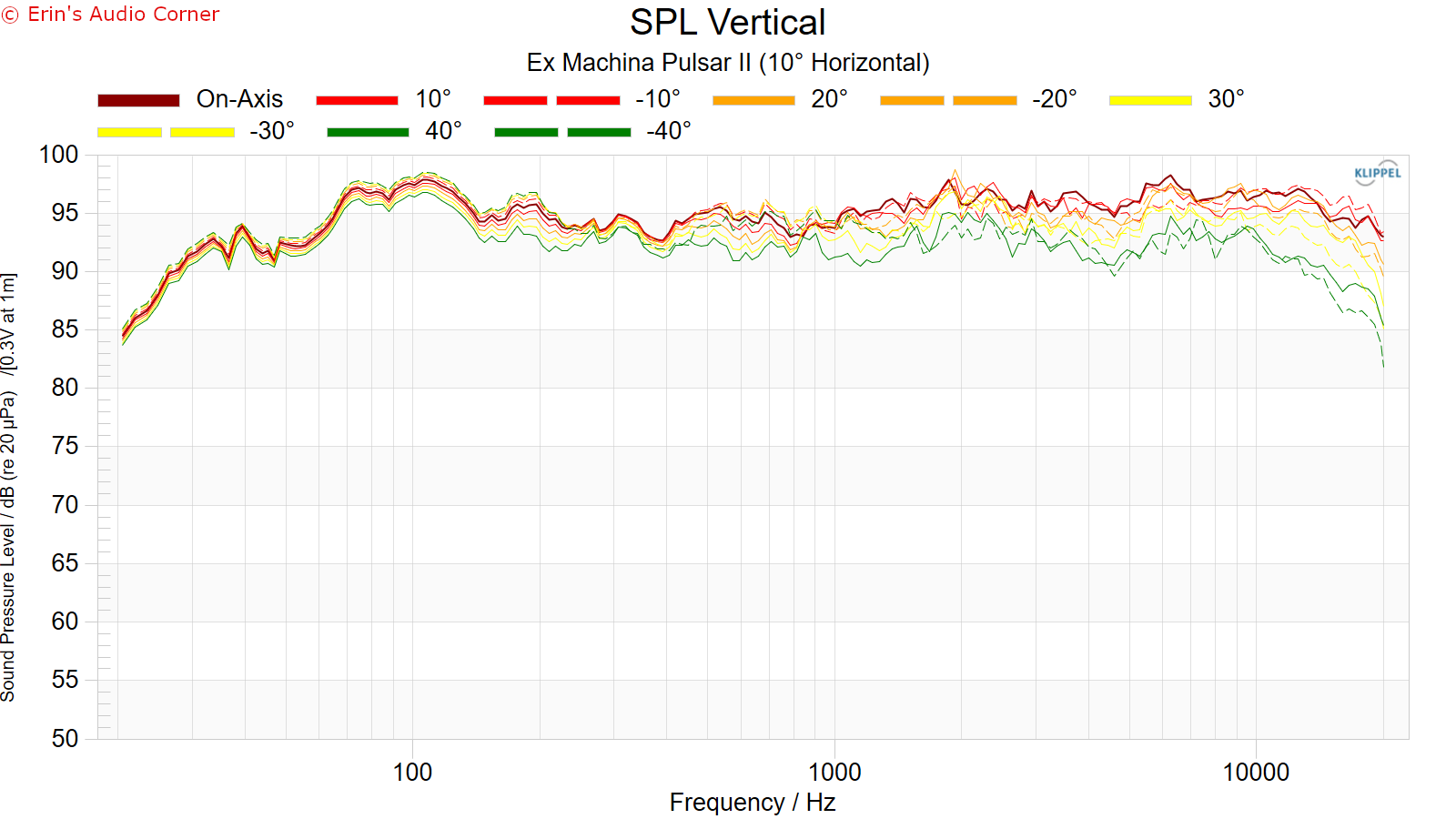
Vertical Frequency Response (0° to ±40°):

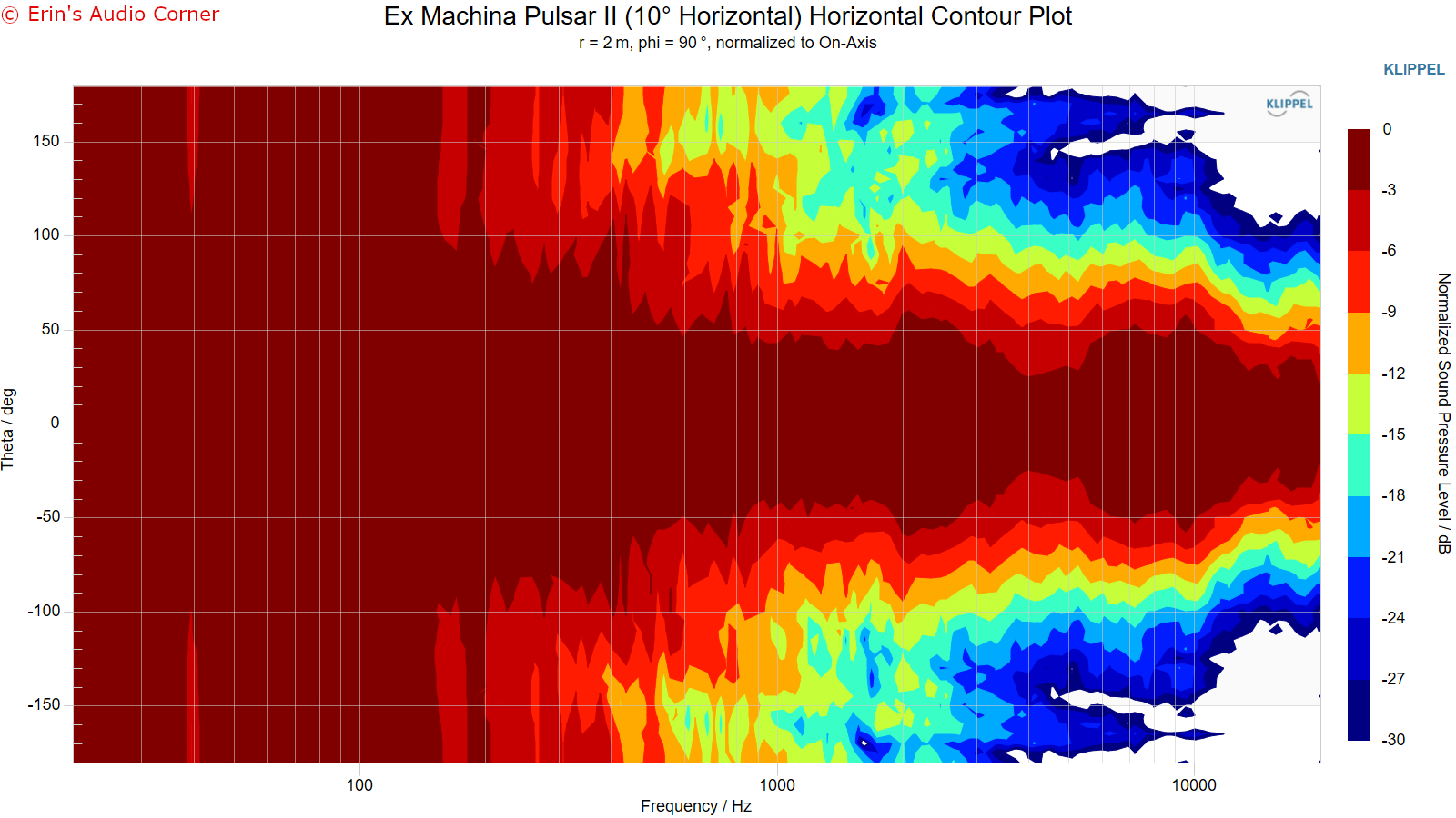
Horizontal Contour Plot (normalized):

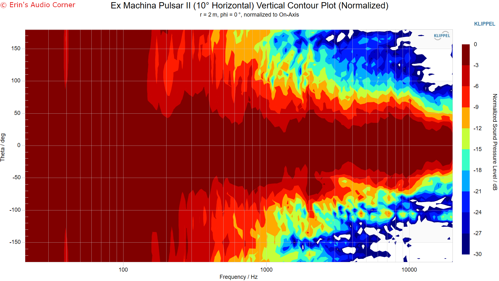
Vertical Contour Plot (normalized):

“Globe” Plots

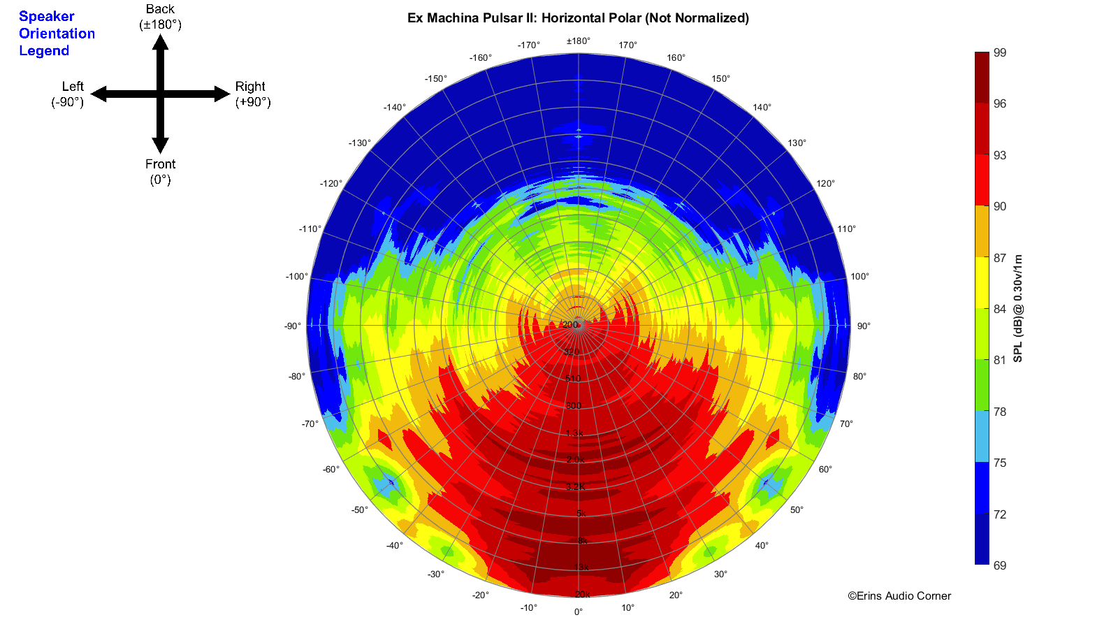
Horizontal Polar (Globe) Plot:
This represents the sound field at 2 meters - above 200Hz - per the legend in the upper left.

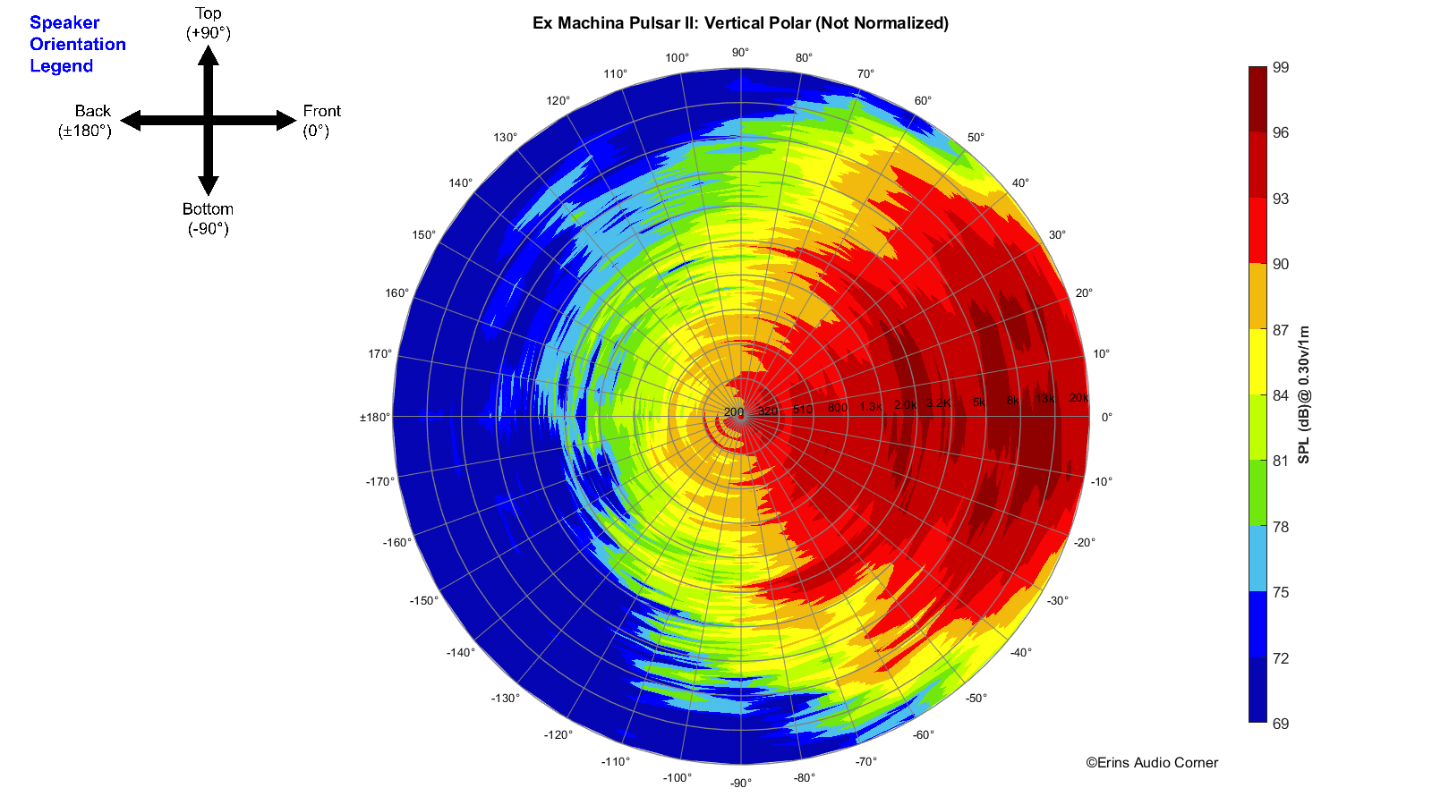
Vertical Polar (Globe) Plot:
This represents the sound field at 2 meters - above 200Hz - per the legend in the upper left.

Additional Measurements

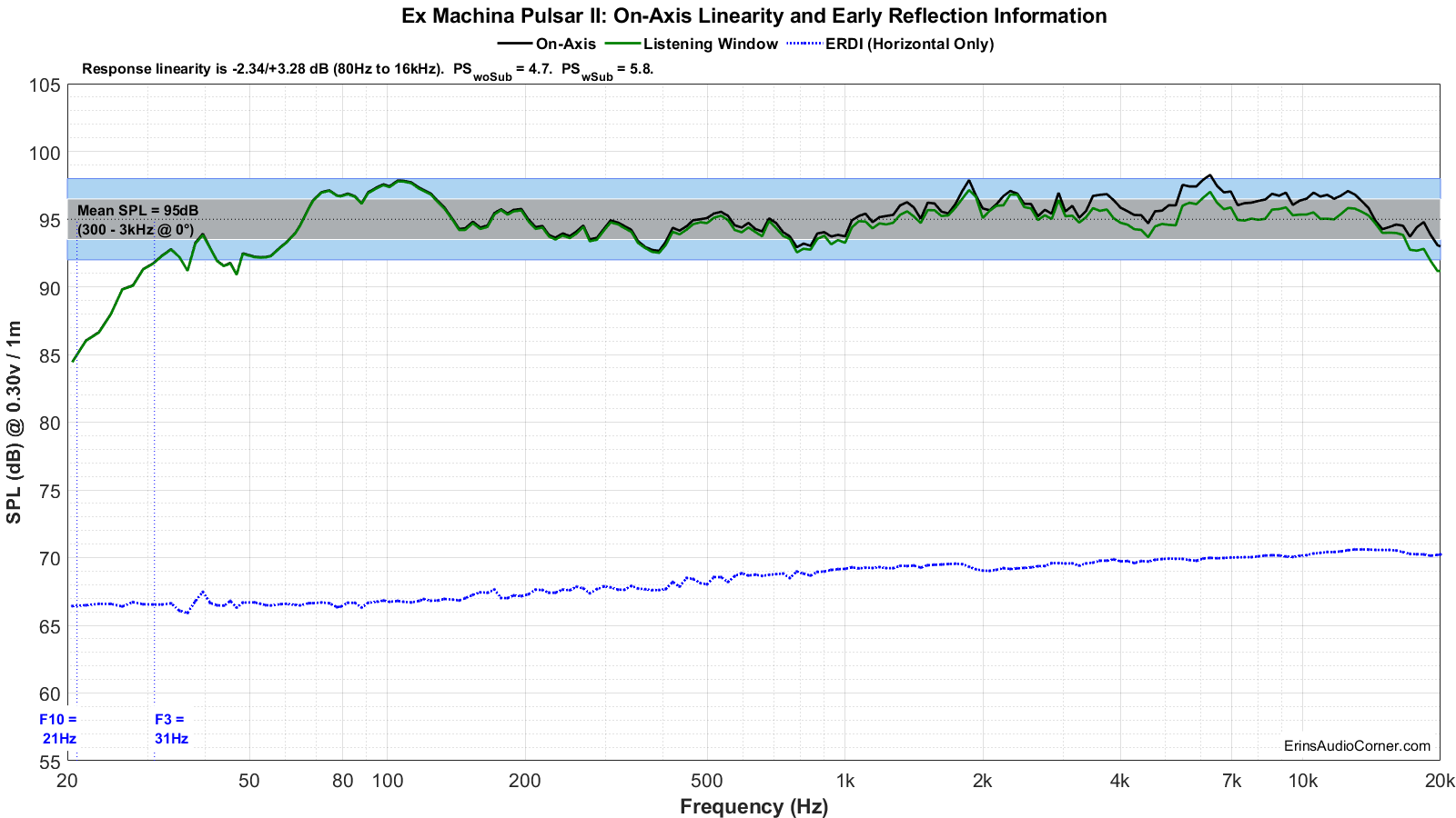
Response Linearity

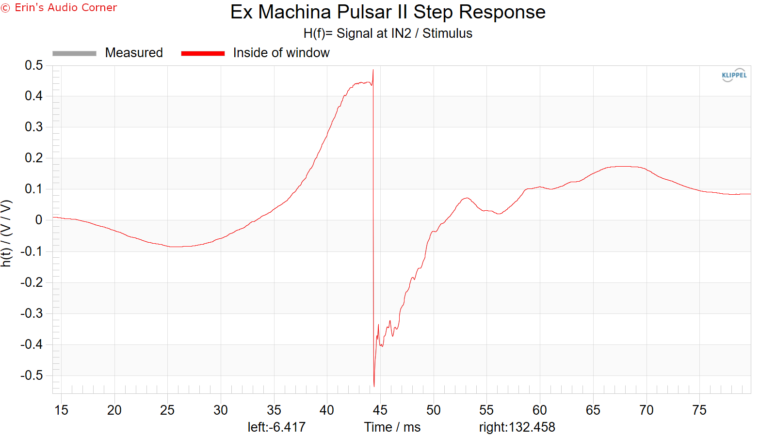
Step Response

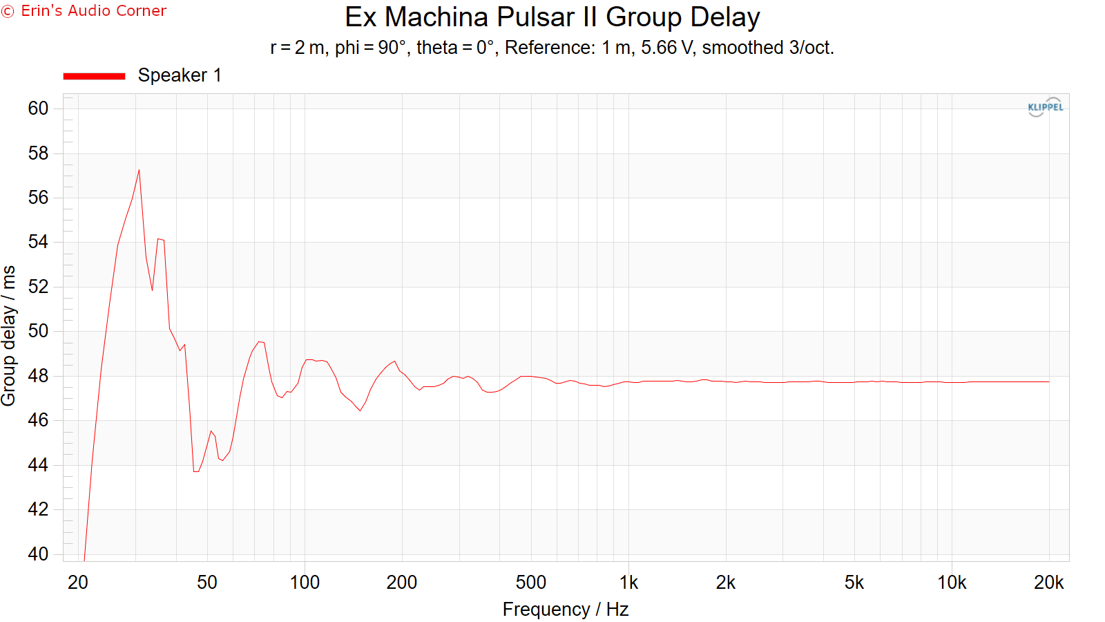
Group Delay

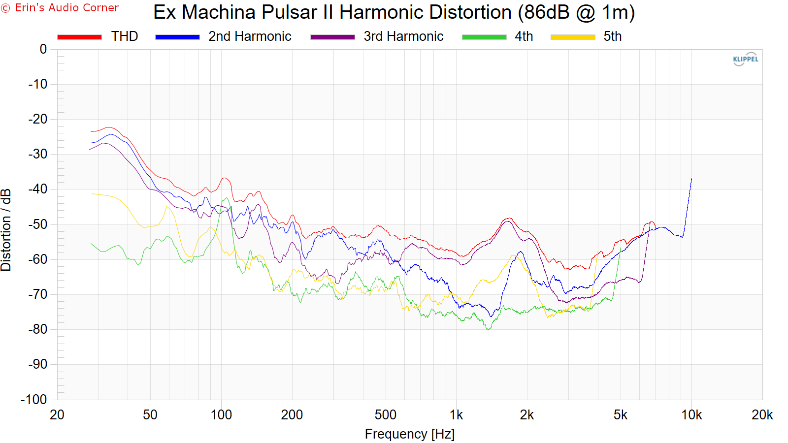
Harmonic Distortion

Harmonic Distortion at 86dB @ 1m:

Harmonic Distortion at 96dB @ 1m:

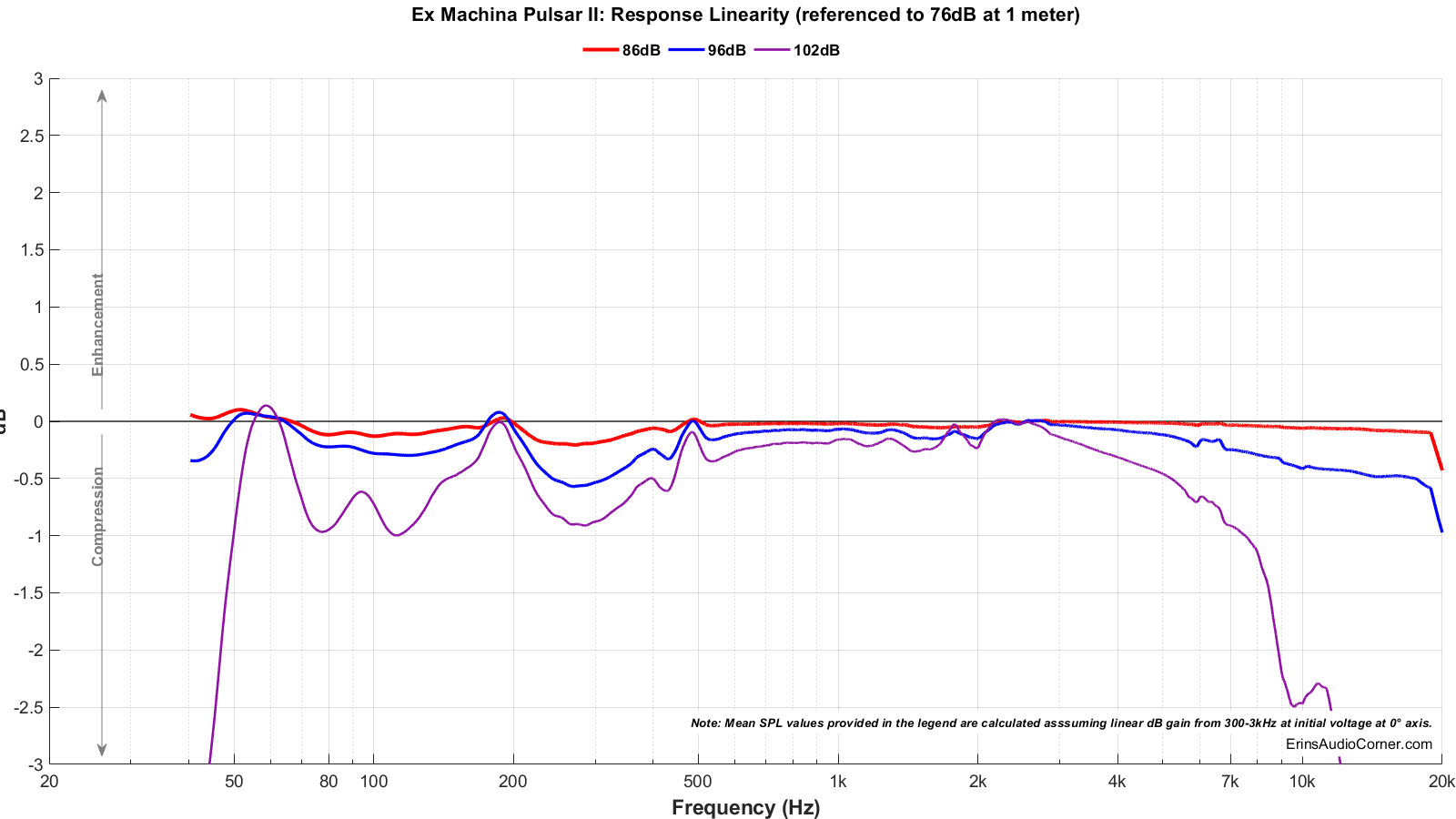
Dynamic Range (Instantaneous Compression Test)

The below graphic indicates just how much SPL is lost (compression) or gained (enhancement; usually due to distortion) when the speaker is played at higher output volumes instantly via a 2.7 second logarithmic sine sweep referenced to 76dB at 1 meter. The signals are played consecutively without any additional stimulus applied. Then normalized against the 76dB result.

The tests are conducted in this fashion:

1. 76dB at 1 meter (baseline; black)
2. 86dB at 1 meter (red)
3. 96dB at 1 meter (blue)
4. 102dB at 1 meter (purple)

The purpose of this test is to illustrate how much (if at all) the output changes as a speaker’s components temperature increases (i.e., voice coils, crossover components) instantaneously.

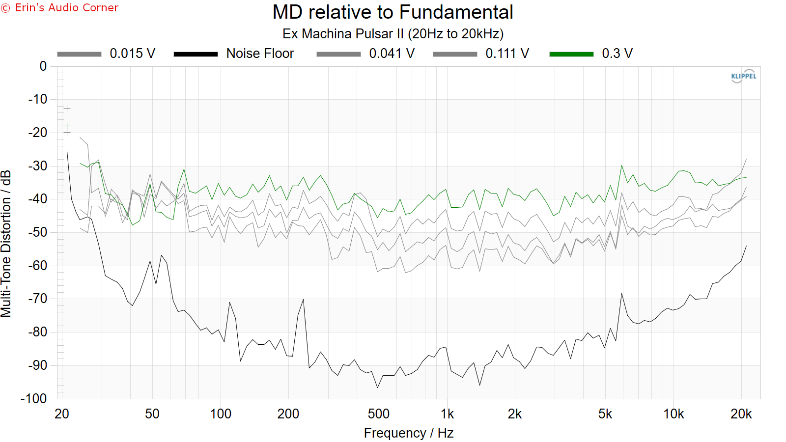
Multitone Distortion

The following tests are conducted at (4) approximate equivalent output volumes: 70/79/87/96dB @ 1 meter. The (4) voltages listed in the legend result in these SPL values.

The test was conducted in (3) manners:

1. Full bandwidth (20Hz to 20kHz)
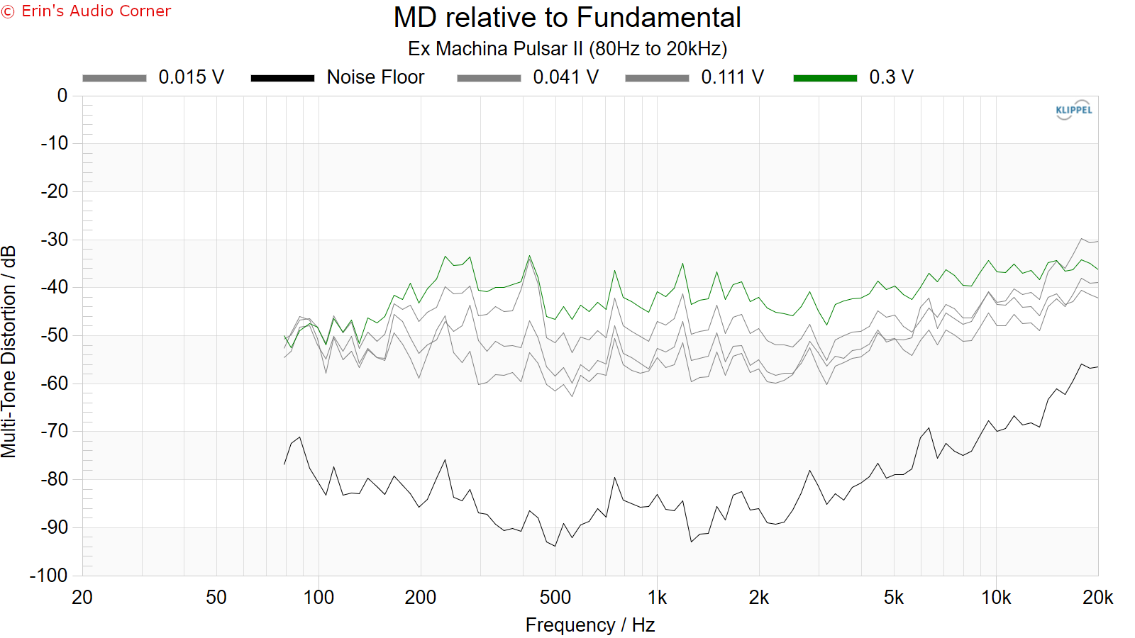
2. 80Hz to 20kHz

The reason for the two measurements is to simulate running the speaker full range vs using a high-pass filter at 80Hz. However, note: the 2nd test low frequency limit at 80Hz is a “brick wall” and doesn’t quite emulate a standard filter of 12 or 24dB/octave. But… it’s close enough.

For information on how to read the below data, watch this video:

1. Full bandwidth (20Hz to 20kHz)

2. 80Hz to 20kHz

Nearfield Measurements (per Ex Machina’s request)”

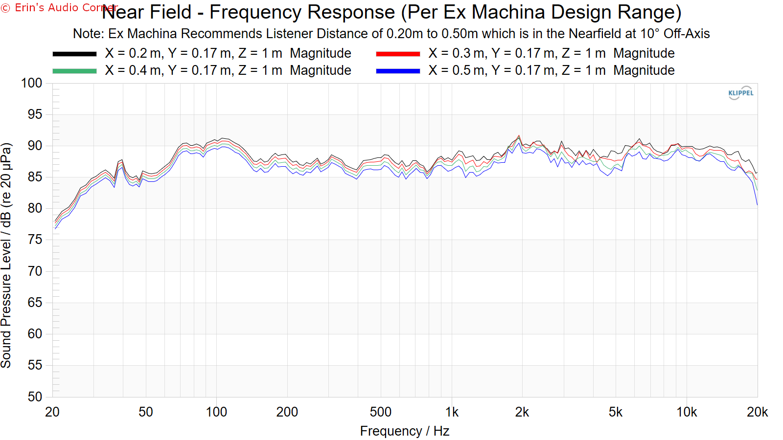
• Black = 0.20 meters listening distance
• Red = 0.30 meters listening distance
• Green = 0.40 meters listening distance
• Blue = 0.50 meters listening distance

Parting / Random Thoughts

See video linked above for subjective and objective analysis. But just a couple notes:

• For the positive, this is one of - if not the best - “3-D” soundstage speakers I’ve heard. In this regard, it’s unparalleled. There is no hard “edge” to the soundstage. Rather, it just extends far in every angle; to the side, front/back and up/down.
• Additionally, the image does a good job of staying parked between the speakers and the tonality is unbothered when moving or shifting positions within a typical headspace (i.e., as you wiggle in your chair or turn to the side to pick up your drink or yell at your kids to turn the music down). This isn’t something I really find necessarily important, per se, but it does give credence to how well aligned the mid and tweeter are aligned at the crossover. Obviously you can’t sit a foot to either side of the speakers and have the same imaging due to time alignment but the timbre is not effected.
• The two above hold true whether you are in the nearfield or the farfield. When it comes to linearity of response of this speaker, however, is where I have issues. There is an obvious audible (and certainly measurable) bass bump about an octave wide - centered at 100Hz - from about 70Hz to 140Hz and a mild “trough” to the midrange. There is evidence of some sort of resonance at around 40Hz in both the nearfield and farfield measurements that was problematic.
• While the overall response above 50Hz is within ±3dB, the midrange and treble are less linear than I’d have hoped for, having a smoothness of about -2.34dB/+3.28dB from 80Hz to 16kHz.
• Directivity is excellent on this speaker. Both vertical and horizontal. I did use my computer to add some equalization tweaks and this speaker responded as well as one would hope. But with that said, the only real EQ tweak I found I had to make was to bring down the ~100Hz-centered bump and smooth out the bass below this.
• In terms of output this speaker has some sort of limiting (either mechanical or DSP) at the highest output volumes. Having said that, if one is listening to a pair of these in the nearfield at 0.50 meters, the 102dB compression results is more analogous to listening at 110dB; something no one in their right mind would ever do. This speaker will otherwise have no issue at all getting you to typical listening volumes of 80dB with 20dB dynamic range.
• Soundstage width for me is rather narrow at about ±40° wide. This is pretty typical of coaxial designs, however, (with the lone exception thus far being the ELAC UBR62 at about ±60°). In the nearfield this is less of a concern.
• With an F3 of 31Hz and F10 of 21Hz, this speaker has plenty of bass output and really makes listening to some of my favorite low bass music quite fun.
• Notably, this speaker has a few selection switches on the back for free-standing and half-space or quarter-space positioning. Basically, this means the bass is shelved a bit for the two latter options if you are placing the speaker near a back wall or in the corner or a room.

While this speaker’s 3-D soundstage was incredible, personally, I think this speaker still needs work. I’d like to see Ex Machina bring down the 100Hz bump by about 2dB and smooth the midrange to get this speaker to “King” status.

Support / Contribute

If you find this review helpful and want to help support the cause that would be AWESOME! There are a few ways you can do so below. Your support helps me pay for new items to test, hardware, miscellaneous items needed for testing, new speakers to review and costs of the site’s server space and bandwidth. Any help is very much appreciated.

Join my Patreon: Become a Patron!

Donate via PayPal:

Shopping

If you are shopping at any of the following stores then please consider using my generic affiliate links below to make the purchase through.

• Amazon
• Audio Advice
• Best Buy
• Crutchfield
• Emotiva
• Monoprice
• Parts Express
• SVS
• Arendal Sound

Purchases through these links can earn me a small commission - at no additional cost to you - and help me continue to provide the community with free content and reviews. Doesn’t matter if it’s a TV from Crutchfield, budget speakers from Audio Advice or a pair of socks from Amazon, just use the link above before you make your purchase. Thank you!