Foreword / YouTube Video Review

The review on this website is a brief overview and summary of the objective performance of this speaker. It is not intended to be a deep dive. Moreso, this is information for those who prefer “just the facts” and prefer to have the data without the filler. Due to extremely limited time, I am not providing any subjective evaluation but hope the data will be enough for designers and DIY’ers alike that they can glean useful information.

For a primer on what the data means, please watch my series of videos where I provide in-depth discussion and examples of how to read the graphics presented hereon.

Information and Photos

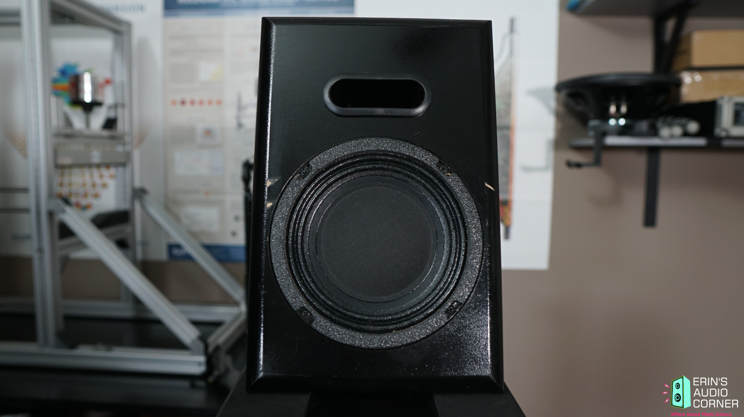
The DIY Sound Group Volt-6 is a DIY design from Matt Grant which is available in kit form from DIYSG. Here are some notes from the product page:

The Volt-6 has a custom made 6.5” coaxial using the same magnet and motor assembly as the Volt-8 and Volt-10. It’s not the prettiest woofer out there but if you need a small home theater speaker capable of high output and power handling, this is a good choice. Impressive X-max with a light weight cone gives this speaker a smooth sounding midrange even when played at high levels. The Celestion CDX1-1010 compression driver (tweeter) is installed on the back and fires through a small waveguide in the center of the woofer giving you point source sound and great off axis response. The crossover was designed to give an even response that not only excels for surround sound speaker use, but also for great front speaker performance but really should be paired with subwoofers that can handle the lower bass. The Volt-6 does quite well in small ported enclosures between .3 and .5cuft when used with a subwoofer. The Atmos version is a small sealed enclosure designed to play down to 115hz, which is perfect for Atmos use. You can use the Volt-6 in your ceiling without an enclosure for Atmos use if needed. For surround sound or mains, you should build the ported models.

These speakers were loaned to me by their owner, who built them from the kit.

CTA-2034 (SPINORAMA) and Accompanying Data

All data collected using Klippel’s Near-Field Scanner. The Near-Field-Scanner 3D (NFS) offers a fully automated acoustic measurement of direct sound radiated from the source under test. The radiated sound is determined in any desired distance and angle in the 3D space outside the scanning surface. Directivity, sound power, SPL response and many more key figures are obtained for any kind of loudspeaker and audio system in near field applications (e.g. studio monitors, mobile devices) as well as far field applications (e.g. professional audio systems). Utilizing a minimum of measurement points, a comprehensive data set is generated containing the loudspeaker’s high resolution, free field sound radiation in the near and far field. For a detailed explanation of how the NFS works and the science behind it, please watch the below discussion with designer Christian Bellmann:

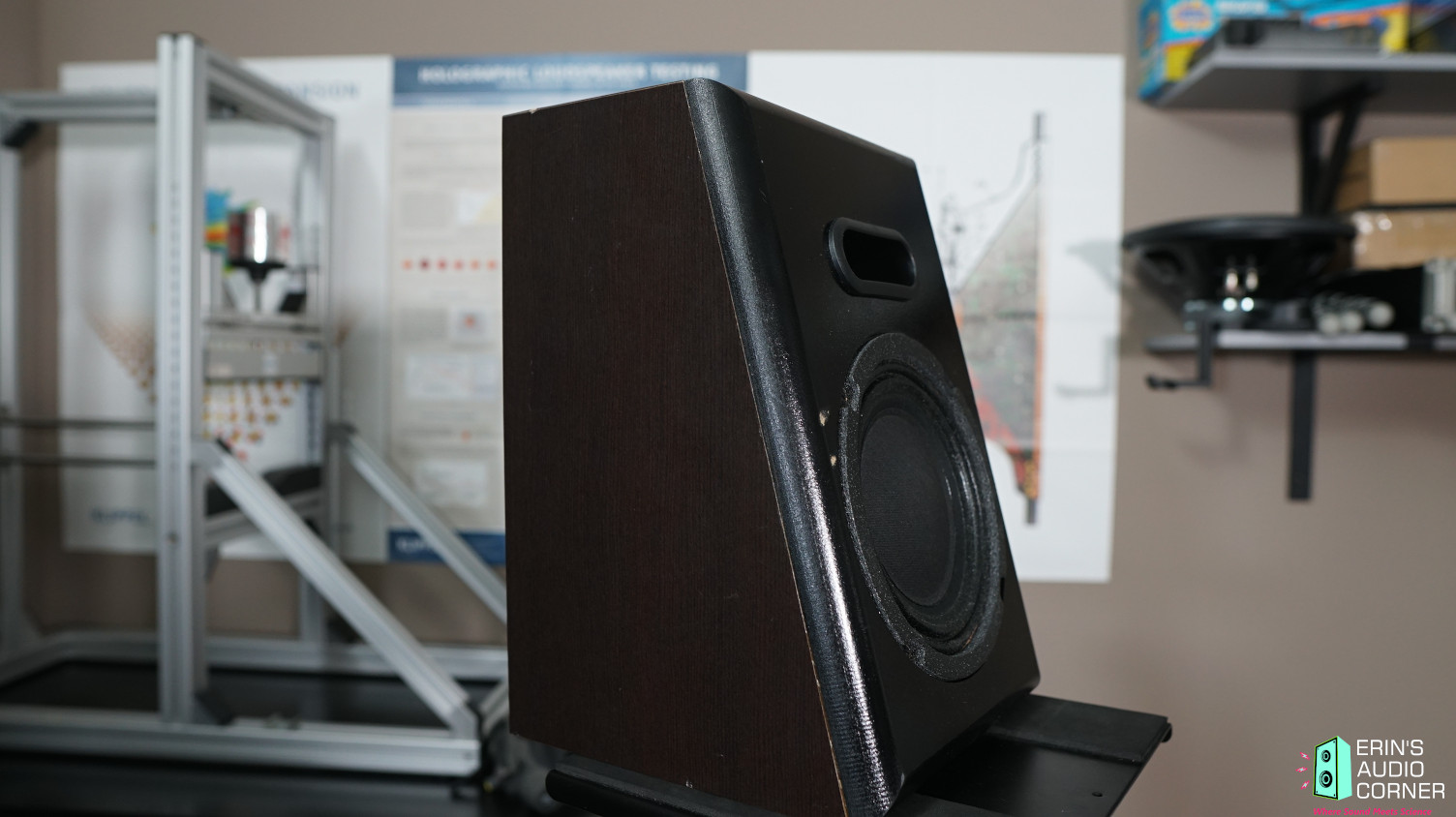
The baffle is sloped at about a 76° angle which made it a bit tricky to measure but after some reconfiguring in the Klippel software, the reference axis was at the tweeter, at the same angle of the baffle.

Measurements are provided in a format in accordance with the Standard Method of Measurement for In-Home Loudspeakers (ANSI/CTA-2034-A R-2020). For more information, please see this link.

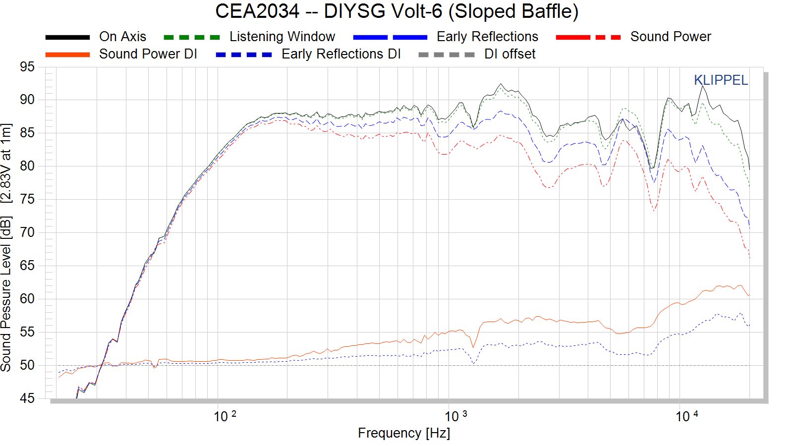
CTA-2034 / SPINORAMA:

The On-axis Frequency Response (0°) is the universal starting point and in many situations, it is a fair representation of the first sound to arrive at a listener’s ears.

The Listening Window is a spatial average of the nine amplitude responses in the ±10º vertical and ±30º horizontal angular range. This encompasses those listeners who sit within a typical home theater audience, as well as those who disregard the normal rules when listening alone.

The Early Reflections curve is an estimate of all single-bounce, first-reflections, in a typical listening room.

Sound Power represents all the sounds arriving at the listening position after any number of reflections from any direction. It is the weighted rms average of all 70 measurements, with individual measurements weighted according to the portion of the spherical surface that they represent.

Sound Power Directivity Index (SPDI): In this standard the SPDI is defined as the difference between the listening window curve and the sound power curve.

Early Reflections Directivity Index (EPDI): is defined as the difference between the listening window curve and the early reflections curve. In small rooms, early reflections figure prominently in what is measured and heard in the room so this curve may provide insights into potential sound quality.

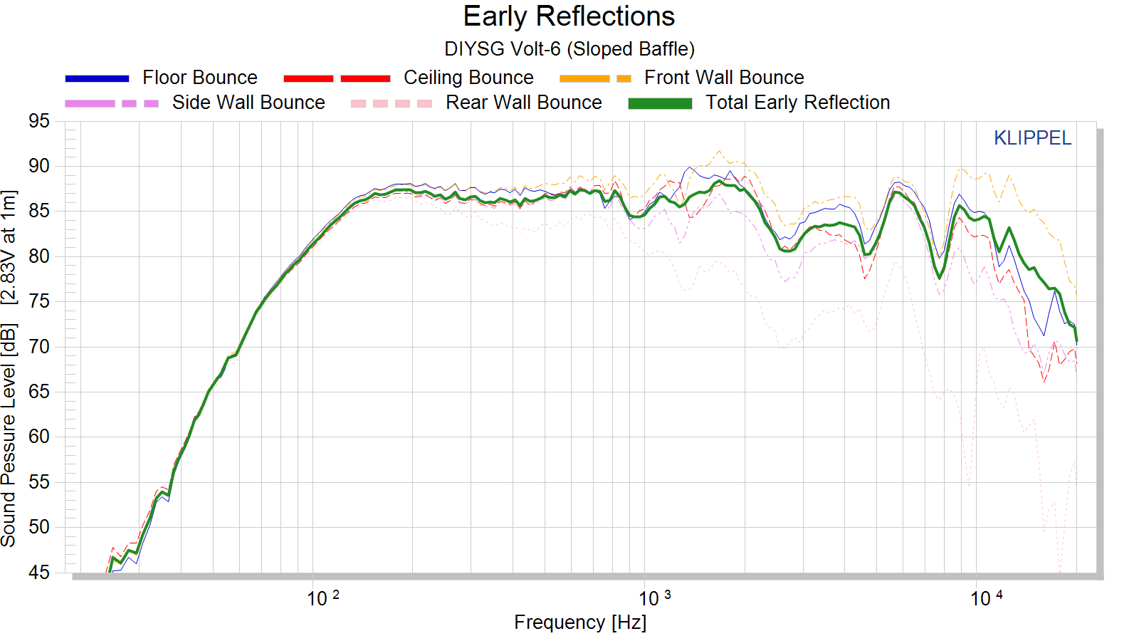
Early Reflections Breakout:

Floor bounce: average of 20º, 30º, 40º down

Ceiling bounce: average of 40º, 50º, 60º up

Front wall bounce: average of 0º, ± 10º, ± 20º, ± 30º horizontal

Side wall bounces: average of ± 40º, ± 50º, ± 60º, ± 70º, ± 80º horizontal

Rear wall bounces: average of 180º, ± 90º horizontal

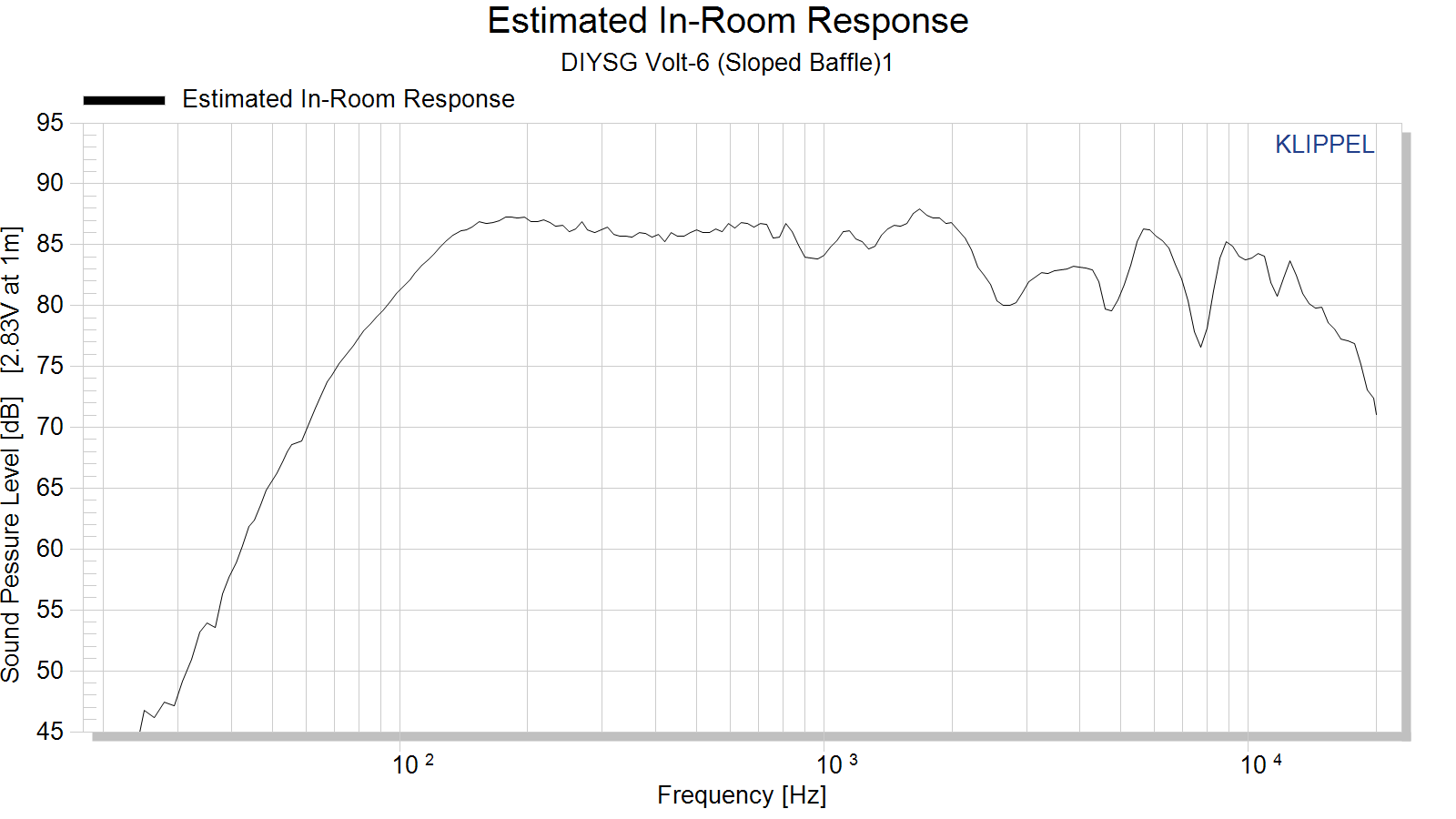
Estimated In-Room Response:

In theory, with complete 360-degree anechoic data on a loudspeaker and sufficient acoustical and geometrical data on the listening room and its layout it would be possible to estimate with good precision what would be measured by an omnidirectional microphone located in the listening area of that room. By making some simplifying assumptions about the listening space, the data set described above permits a usefully accurate preview of how a given loudspeaker might perform in a typical domestic listening room. Obviously, there are no guarantees because individual rooms can be acoustically aberrant. Sometimes rooms are excessively reflective (“live”) as happens in certain hot, humid climates, with certain styles of interior décor and in under-furnished rooms. Sometimes rooms are excessively “dead” as in other styles of décor and in some custom home theaters where acoustical treatment has been used excessively. This form of post processing is offered only as an estimate of what might happen in a domestic living space with carpet on the floor and a “normal” amount of seating, drapes, and cabinetry.

For these limited circumstances it has been found that a usefully accurate Predicted In-Room (PIR) amplitude response, also known as a “room curve” is obtained by a weighted average consisting of 12 % listening window, 44 % early reflections and 44 % sound power. At very high frequencies errors can creep in because of excessive absorption, microphone directivity, and room geometry. These discrepancies are not considered to be of great importance.

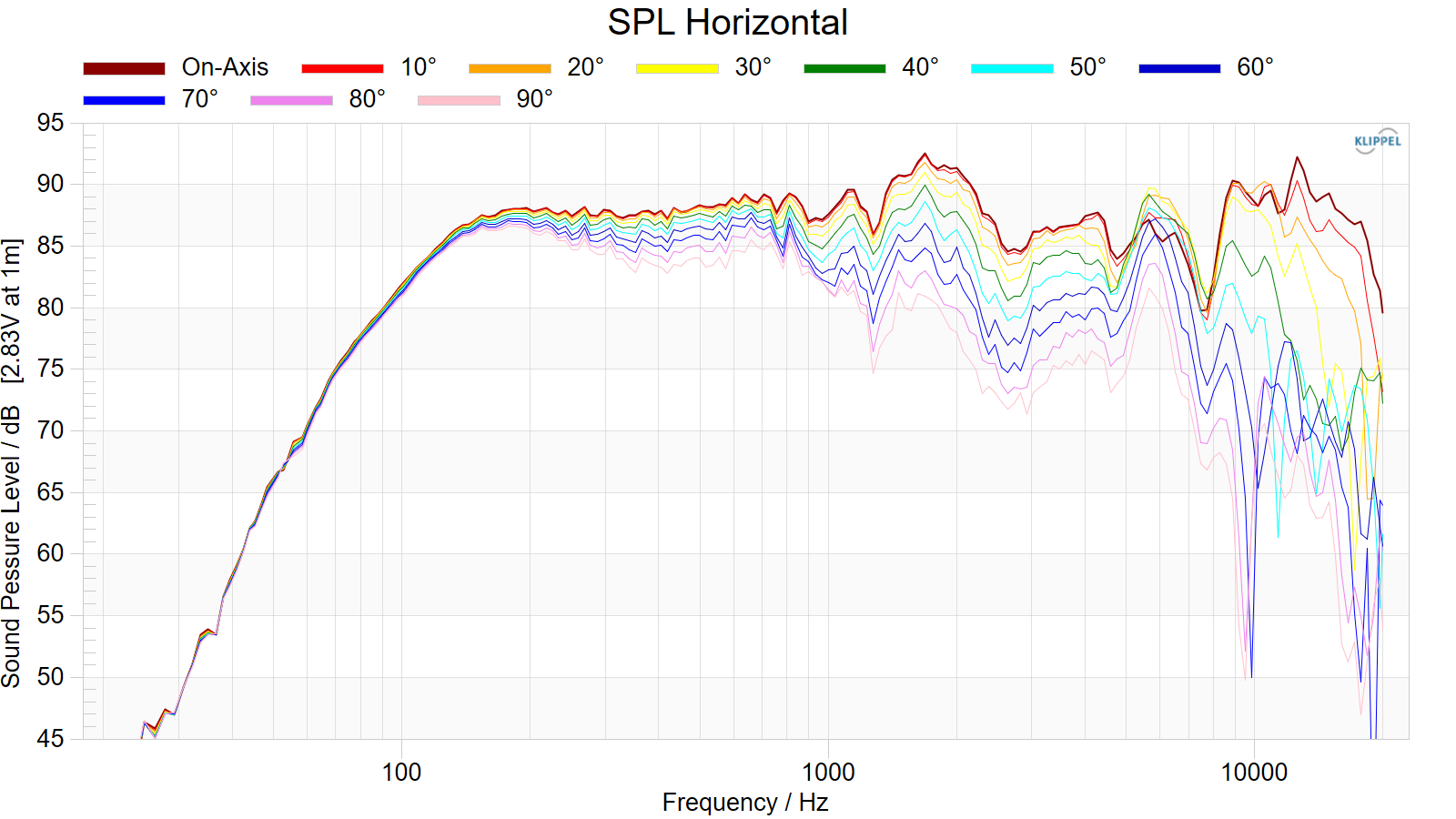
Horizontal Frequency Response (0° to ±90°):

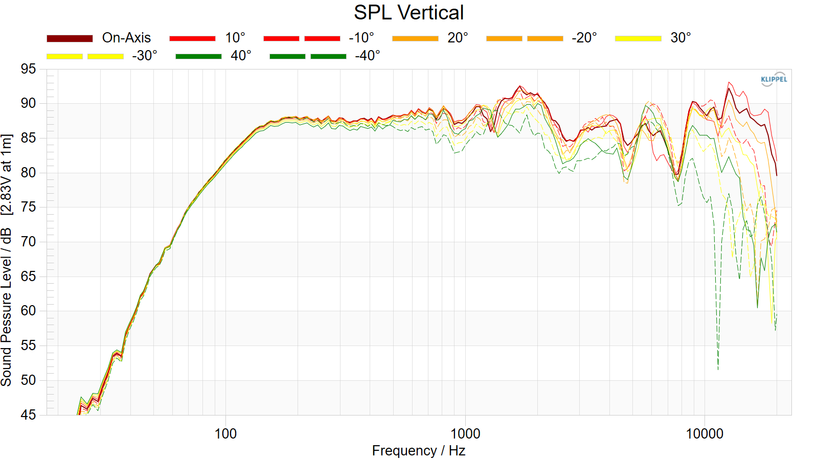
Vertical Frequency Response (0° to ±40°):

Horizontal Contour Plot (not normalized):

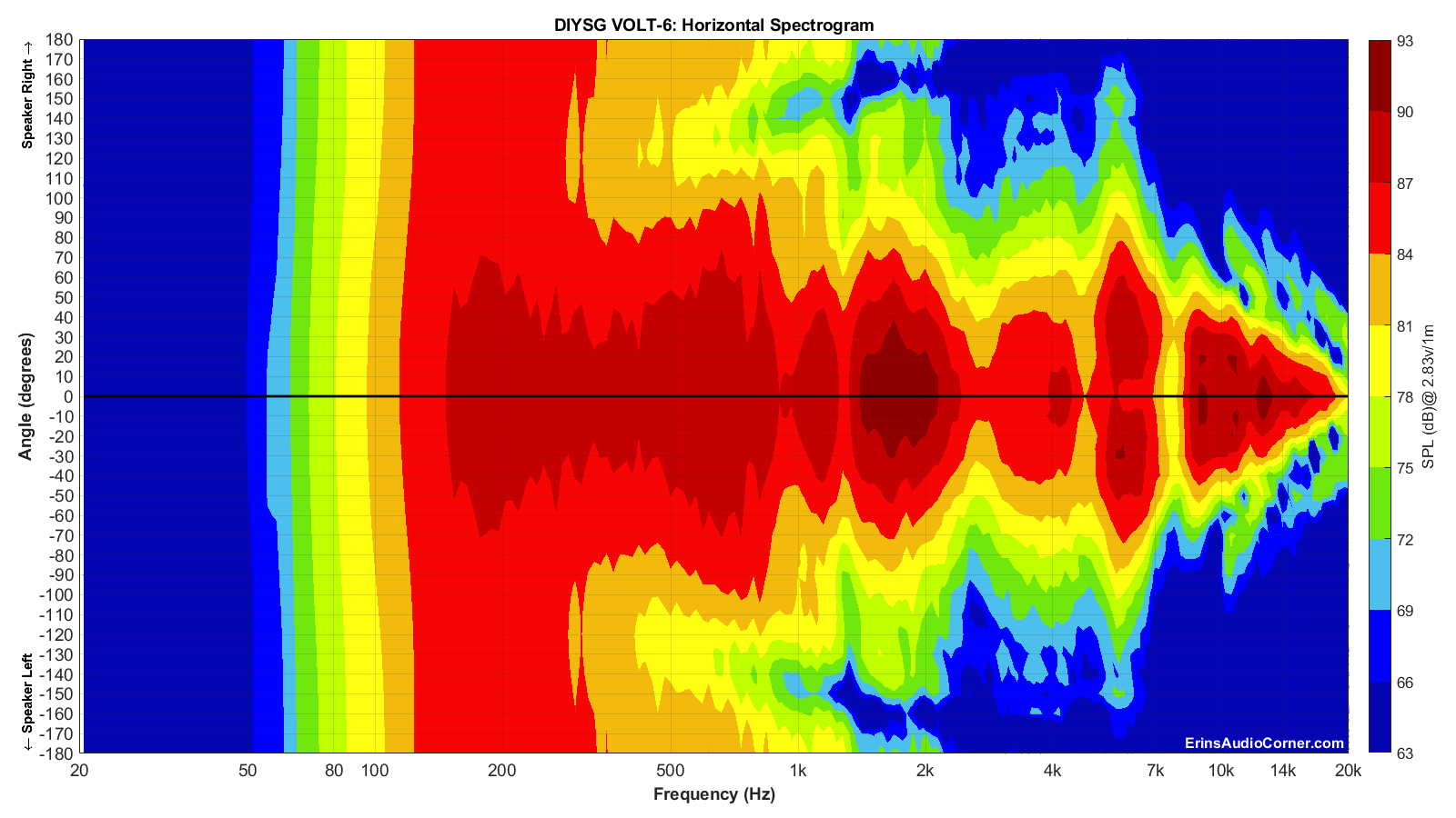
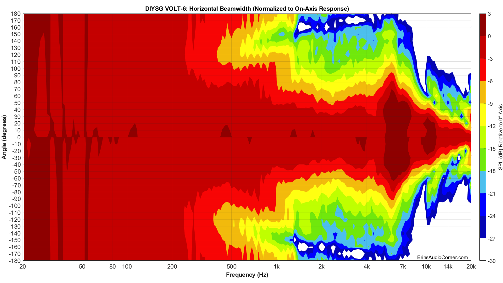
Horizontal Contour Plot (normalized):

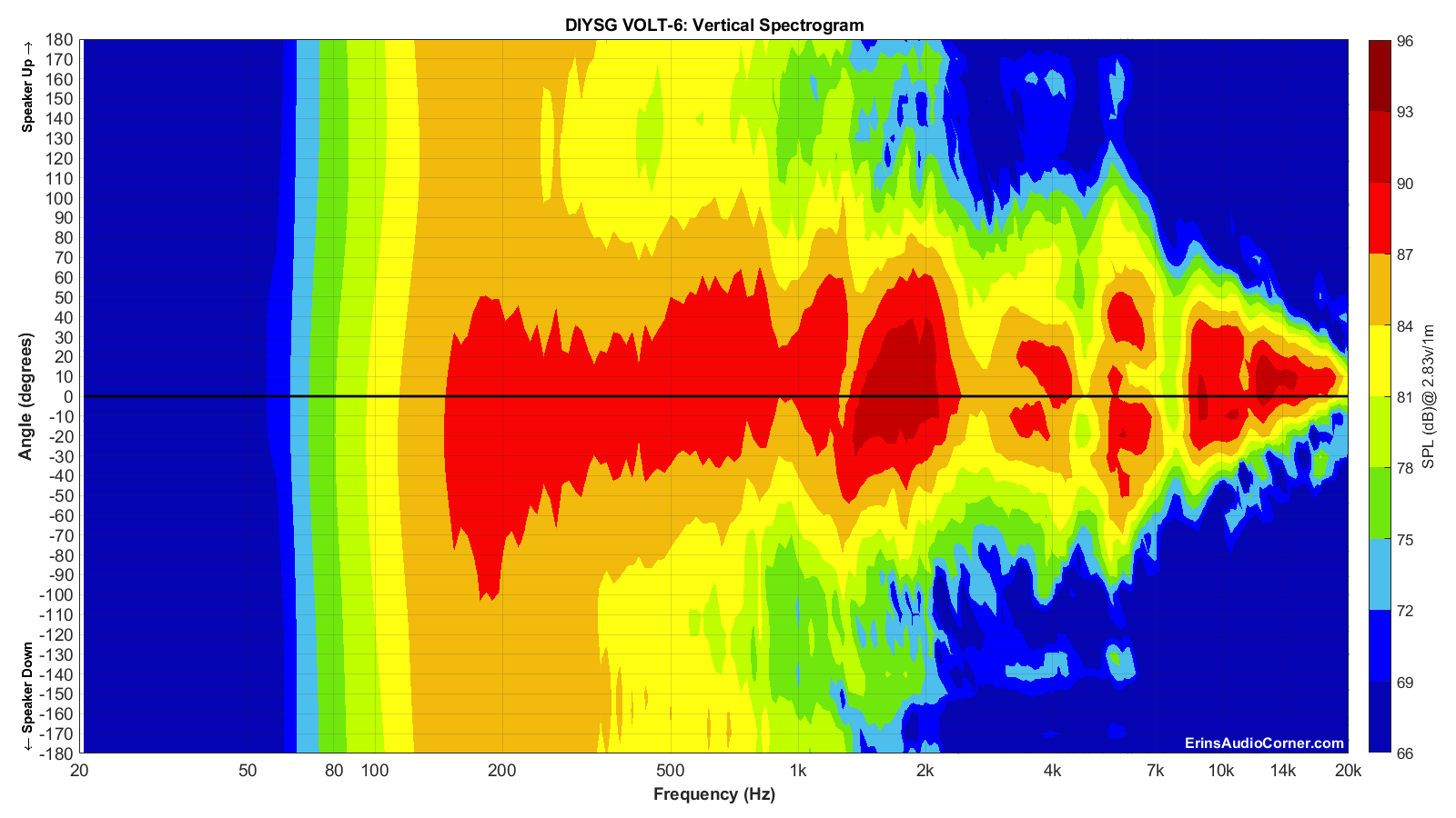
Vertical Contour Plot (not normalized):

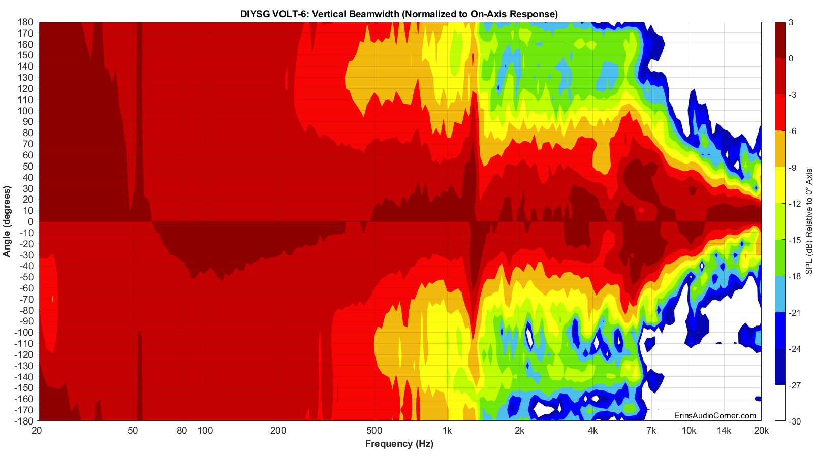
Vertical Contour Plot (normalized):

Additional Measurements

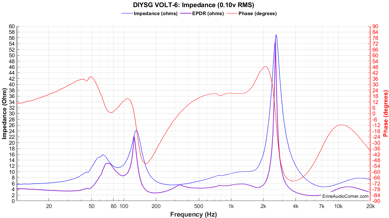
Impedance Magnitude and Phase + Equivalent Peak Dissipation Resistance (EPDR)

For those who do not know what EPDR is (ahem, me until 2020), Keith Howard came up with this metric which he defined in a 2007 article for Stereophile as:

… simply the resistive load that would give rise to the same peak device dissipation as the speaker itself.

A note from Dr. Jack Oclee-Brown of Kef (who supplied the formula for calculating EPDR):

Just a note of caution that the EPDR derivation is based on a class-B output stage so it’s valid for typical class-AB amps but certainly not for class-A and probably has only marginal relevance for class-D amps (would love to hear from a class-D expert on this topic).

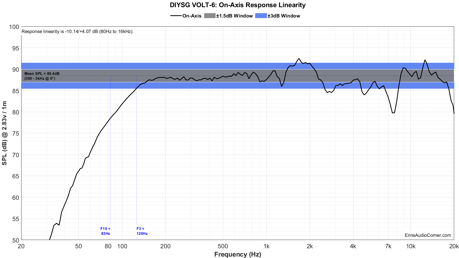
On-Axis Response Linearity

“Globe” Plots

These plots are generated from exporting the Klippel data to text files. I then process that data with my own MATLAB script to provide what you see. These are not part of any software packages and are unique to my tests.

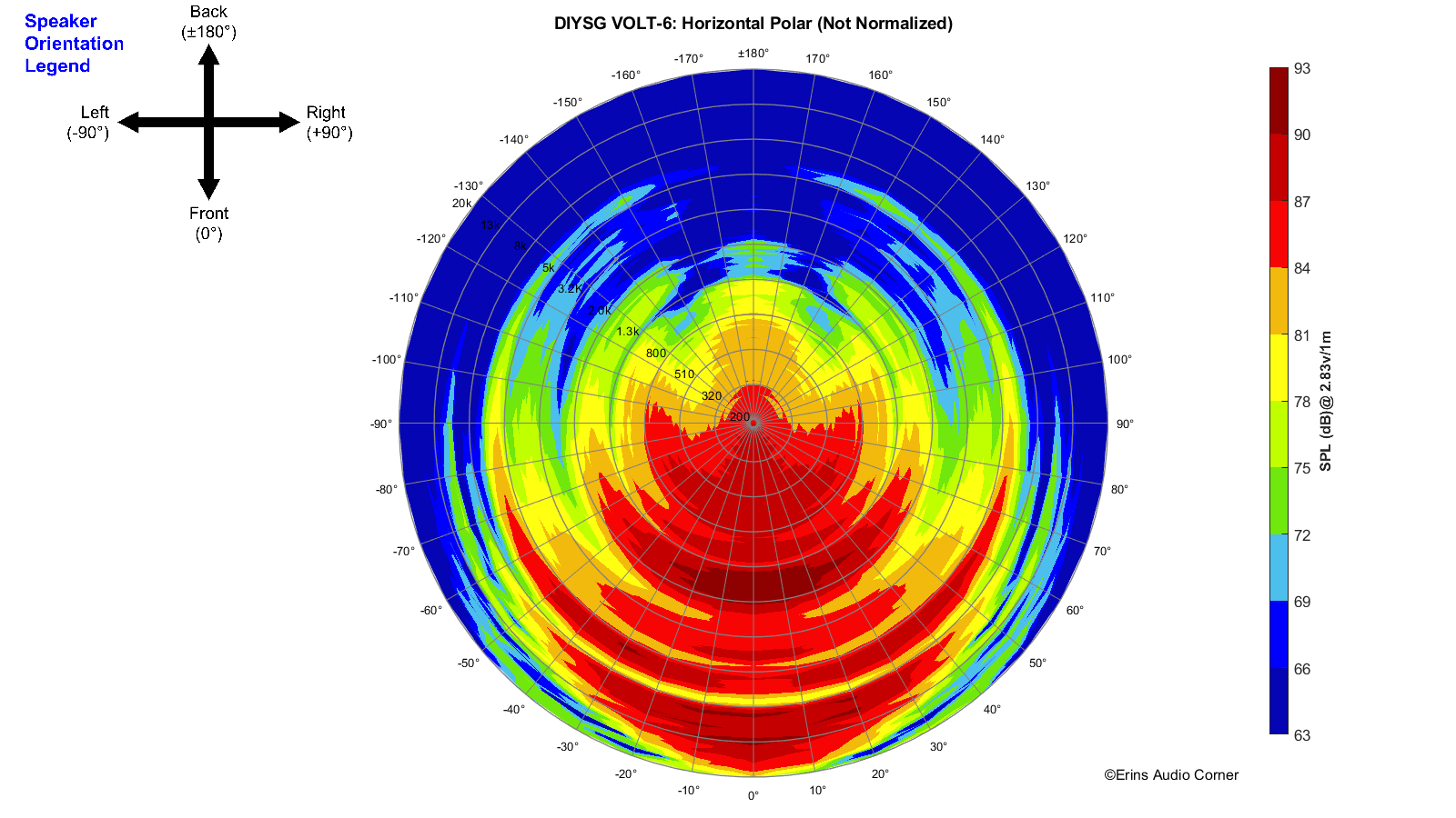
Horizontal Polar (Globe) Plot:
This represents the sound field at 2 meters - above 200Hz - per the legend in the upper left.

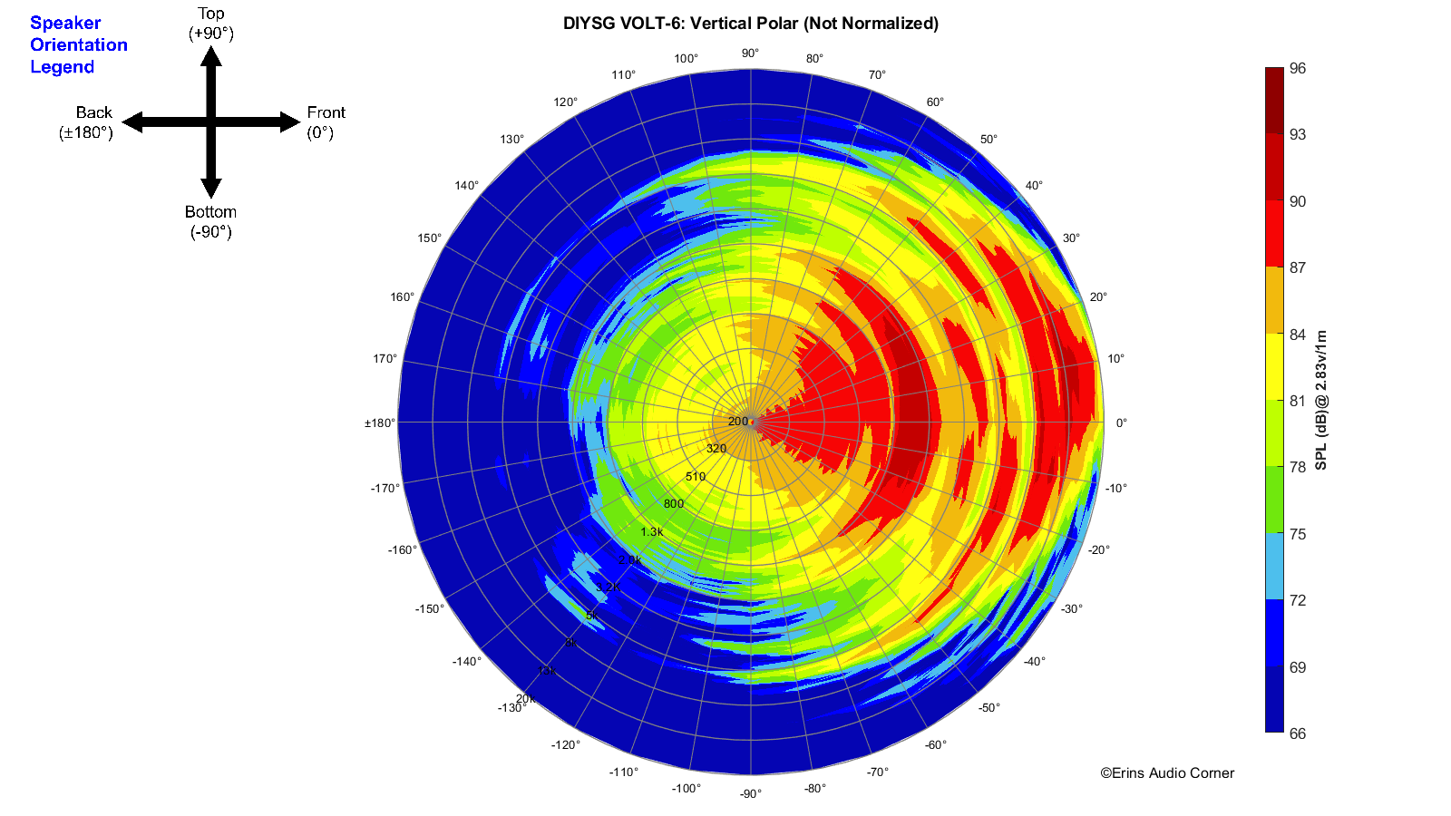
Vertical Polar (Globe) Plot:
This represents the sound field at 2 meters - above 200Hz - per the legend in the upper left.

Harmonic Distortion

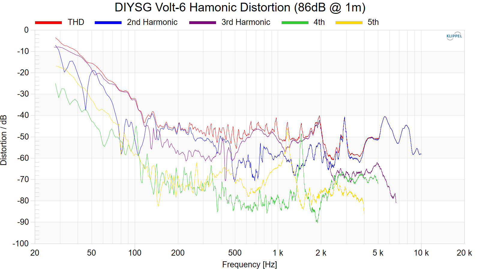
Harmonic Distortion at 86dB @ 1m:

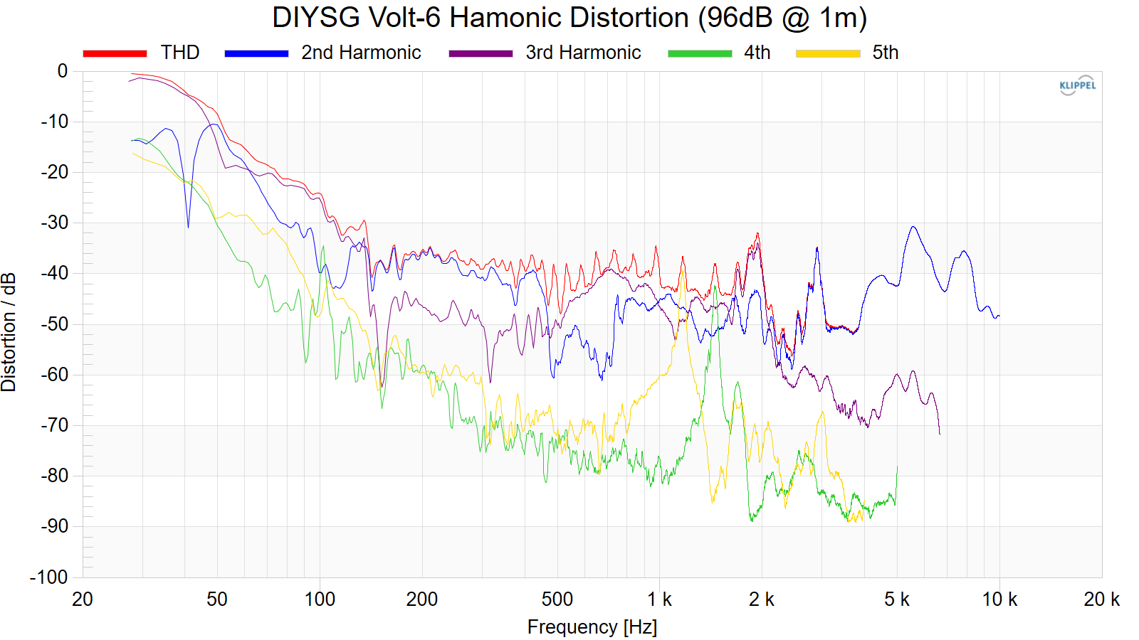
Harmonic Distortion at 96dB @ 1m:

Dynamic Range (Instantaneous Compression Test)

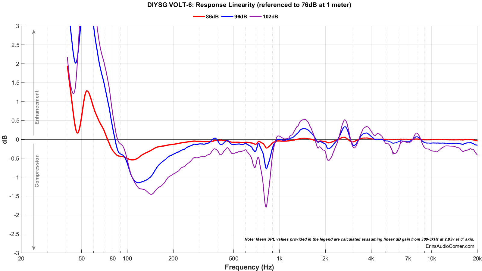
The below graphic indicates just how much SPL is lost (compression) or gained (enhancement; usually due to distortion) when the speaker is played at higher output volumes instantly via a 2.7 second logarithmic sine sweep referenced to 76dB at 1 meter. The signals are played consecutively without any additional stimulus applied. Then normalized against the 76dB result.

The tests are conducted in this fashion:

1. 76dB at 1 meter (baseline; black)
2. 86dB at 1 meter (red)
3. 96dB at 1 meter (blue)
4. 102dB at 1 meter (purple)

The purpose of this test is to illustrate how much (if at all) the output changes as a speaker’s components temperature increases (i.e., voice coils, crossover components) instantaneously.

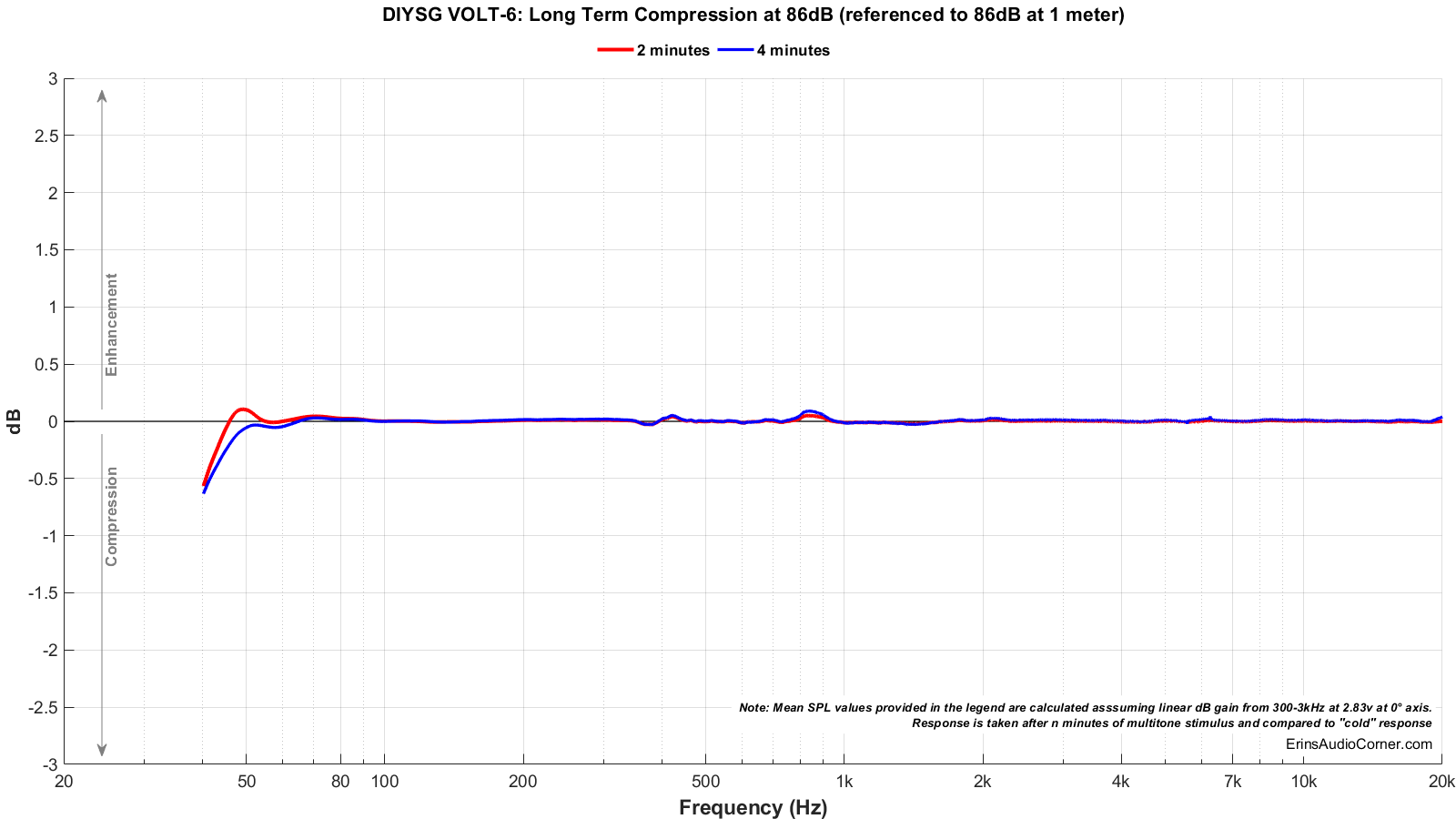
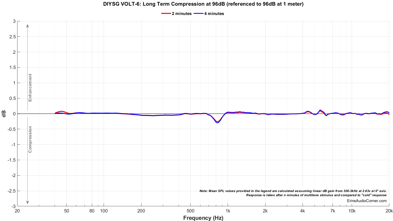
Long Term Compression Tests

The below graphics indicate how much SPL is lost or gained in the long-term as a speaker plays at the same output level for 2 minutes, in intervals. Each graphic represents a different SPL: 86dB and 96dB both at 1 meter.

The purpose of this test is to illustrate how much (if at all) the output changes as a speaker’s components temperature increases (i.e., voice coils, crossover components).

The tests are conducted in this fashion:

1. “Cold” logarithmic sine sweep (no stimulus applied beforehand)
2. Multitone stimulus played at desired SPL/distance for 2 minutes; intended to represent music signal
3. Interim logarithmic sine sweep (no stimulus applied beforehand) (Red in graphic)
4. Multitone stimulus played at desired SPL/distance for 2 minutes; intended to represent music signal
5. Final logarithmic sine sweep (no stimulus applied beforehand) (Blue in graphic)

The red and blue lines represent changes in the output compared to the initial “cold” test.

Placement Consideration (Effect of On-Wall Installation)

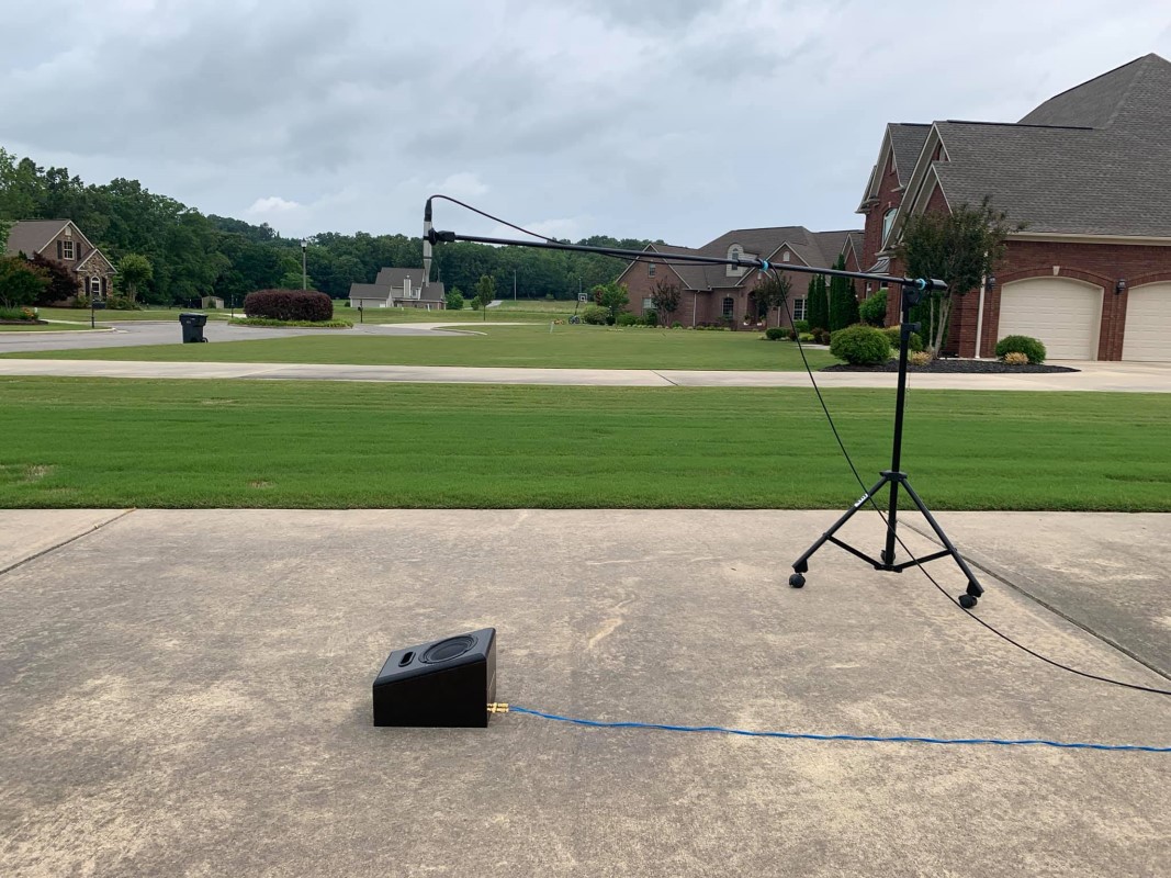
Many people seem to be using this speaker as an on-wall speaker for surround use. Therefore, the anechoic data - data taken in free space - is not fully representative of the Volt-6’s on-wall performance. Therefore, I placed the speaker outside on the ground, facing up. I placed the microphone on a boom and positioned the microphone 1 meter above the speaker as illustrated in the photograph below.

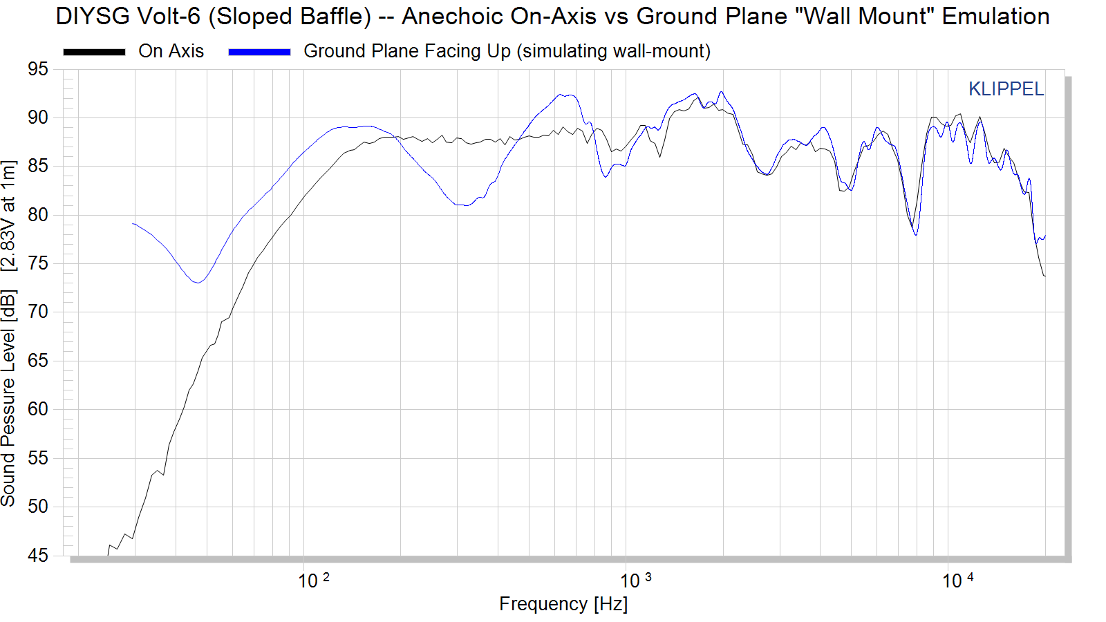
I have provided an overlay of the SPINORAMA’s on-axis response (black) vs the “Wall Mount” measurement (blue) below. This is intended to be a caution that speakers which are not specifically designed for on-wall use will result in fairly significant comb filtering so be advised of this.

Parting / Random Thoughts

• Measured sensitivity averages approximately 88.4dB @ 1m.
• I’m really surprised at the Dynamic Range and Compression test results. There is a significant amount of distortion below 100Hz which causes enhancement (solidified by simply looking at the harmonic distortion graphic). Above 100Hz through about 1kHz there is a good bit of compression. That all said, the long-term compression testing doesn’t look as bad. Just realize that the difference in frequency response is going to be quite different as you increase volume. Using an appropriate highpass filter (I’d estimate 100Hz or greater) will help this but not solve the issues.
• The response linearity is pretty poor. If I am being honest, this just seems like a sub-par coaxial driver with poor tweeter/mid integration. I say that because the 6kHz region shows some sort of issue where the off-axis response is even higher in SPL than the on-axis response; something I typically see in waveguides and this is way above the crossover point. There are also pretty significant combing effects above this, especially above 10kHz.
• There is a resonance around 800Hz (evidenced by the impedance blip, the “stacking” of frequency response magnitude and the increased compression, the latter of which is typically a sign of port resonance).
• Remember what I said about wall-mounting this speaker. Ideally, you would flush mount the speaker in the wall or in the ceiling (as the designer suggests). This would help the bass rolloff by providing an “infinite baffle”, reinforcing the lower frequencies. Though, baffle step would need to be properly accounted for.
• Note the vertical axis measurement doesn’t appear to be perfectly aligned with the acoustic center of the speaker. This isn’t for a lack of trying. I re-measured the speaker a few times, adjusting the reference point each time. Judging by the contour data, each measurement was either just above or just below the dead-center vertical alignment which makes me think that one of those angles I used was correct; there is just a good deal of comb filtering going on causing the high frequency measurements >10kHz to look out of sorts. What I have provided here is the best guesstimate at what is the correct angle for the angle of the baffle.
• The vent tuning frequency seems to be off judging by the impedance sweep.

Support / Donate

If you like what you see here and want to help me keep it going, please consider donating via the PayPal Contribute button below. Donations help me pay for new items to test, hardware, miscellaneous items and costs of the site’s server space and bandwidth. All of which I pay out of pocket. So, if you can help chip in a few bucks, know that it is very much appreciated and that the support means a lot to me.

Alternatively, if you have a need to purchase anything through Amazon, please consider using my Amazon affiliate link below. It yields me a small commission at no additional cost to you and allows me to keep providing you with sweet data to make educated purchase decisions.

You can also join my Facebook and YouTube pages if you would like to follow along with updates.